Tutorial 18: Topology optimization

In this tutorial, we will learn:

How to apply the adjoint method for sensitivity analysis in Gridap
How to do topology optimization in Gridap

We recommend that you first read the Electromagnetic scattering tutorial to make sure you understand the following points:

How to formulate the weak form for a 2d time-harmonic electromagnetic problem (a scalar Helmholtz equation)
How to implement a perfectly matched layer (PML) to absorb outgoing waves
How to impose periodic boundary conditions in Gridap
How to discretize PDEs with complex-valued solutions

Problem statement

Consider the following optimization problem adapted from Christiansen et al. (2020): We want to design a metallic (silver) nanoparticle to focus an incident $H_z$-polarized planewave on a single spot, maximizing the electric-field intensity at this focal spot. The metallic structure can be any shape of any topology (any connectivity, number of holes, etcetera) surrounding the focal spot, as long as the metal lies within an annular "design region" $\Omega_d$: between a minimum radius $r_s = 10$nm (the minimum distance from the focal spot) and an outer radius $r_d=100$nm. The computational cell is of height $H$ and length $L$, and we employ a perfectly matched layer (PML) thickness of $d_{pml}$ to implement outgoing (radiation) boundary conditions for this finite domain.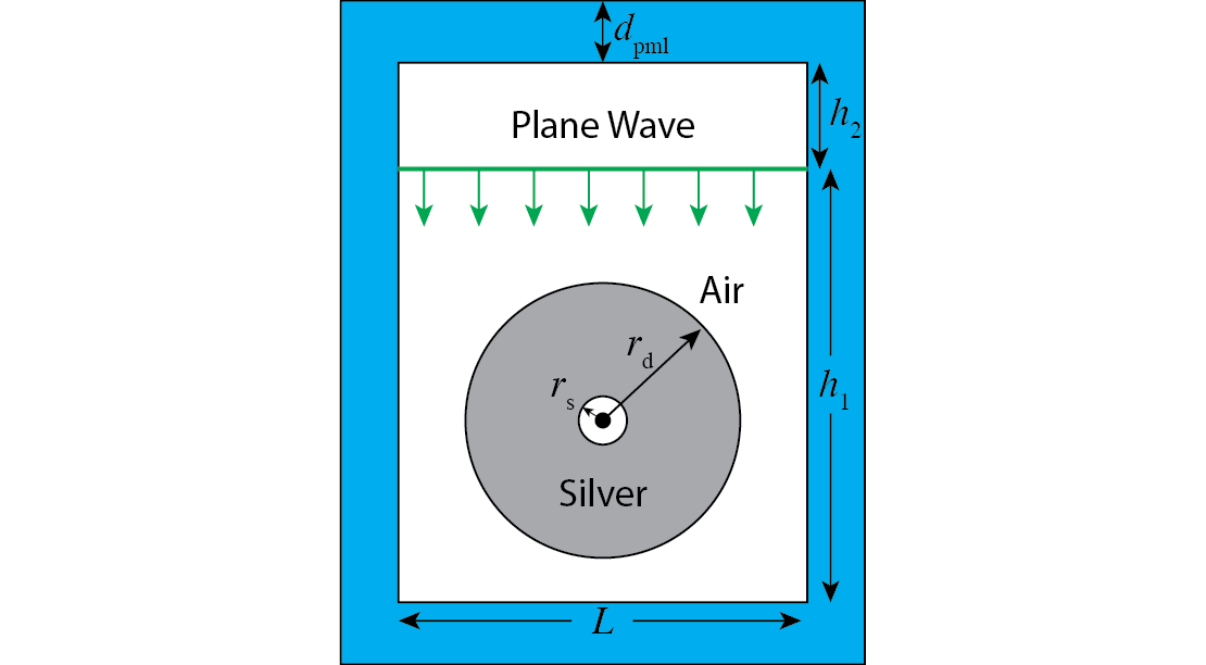

The goal is find the arrangement of the silver material in the gray region that maximizes the |electric field|² at the center (the focal point). Every "pixel" in the gray region is effectively treated as a degree of freedom that can vary continuously between silver (shown in black below) and air (shown in white below). This is called density-based topology optimization (TO), and leads to a tractable optimization problem despite the huge number of parameters. A standard "projection" technique, described below, is used to "binarize" the structure by eventually forcing the material to be either silver or air almost everywhere.

Formulation

From Maxwell's equations, considering a time-harmonic electromagnetic field polarized so that the electric field is in-plane and the magnetic field is out-of-plane (described by a scalar $H$ equal to the z-component), we can derive the governing equation of this problem in 2D (Helmholtz equation) [1]:

\[\left[-\nabla\cdot\frac{1}{\varepsilon(x)}\nabla -k^2\mu(x)\right] H = f(x),\]

where $k=\omega/c$ is the wave number in free space and $f(x)$ is the source term (which corresponds to a magnetic current density in Maxwell's equations).

In order to simulate this scattering problem in a finite computational domain, we need outgoing (radiation) boundary conditions to prevent waves from reflecting back from the boundaries of the domain. We employ the well-known technique of "perfectly matched layers" (PML) [2], which are an an artificial absorbing layer adjacent to the boundaries that absorbs waves with minimal reflections (going to zero as the resolution increases). The "stretched-coordinate" formulation of PML correspond to a simple transformation of the PDE [3]:

\[\frac{\partial}{\partial x}\rightarrow \frac{1}{1+\mathrm{i}\sigma(u_x)/\omega}\frac{\partial}{\partial x},\]

\[\frac{\partial}{\partial y}\rightarrow \frac{1}{1+\mathrm{i}\sigma(u_y)/\omega}\frac{\partial}{\partial y},\]

where $u_{x/y}$ is the depth into the PML, $\sigma$ is a profile function (here we chose $\sigma(u)=\sigma_0(u/d_{pml})^2$) and the $x$ and $y$ derivatives correspond PML layers at the $x$ and $y$ boundaries, respectively. Note that at a finite mesh resolution, PML reflects some waves, and the standard technique to mitigate this is to "turn on" the PML absorption gradually—in this case we use a quadratic profile. The amplitude $\sigma_0$ is chosen so that in the limit of infinite resolution the "round-trip" normal-incidence is some small number.

Since PML absorbs all waves before they reach the boundary, the associated boundary condition can then be chosen arbitrarily. Here, the boundary conditions are Dirichlet (zero) on the top and bottom sides $\Gamma_D$ but periodic on the left ($\Gamma_L$) and right sides ($\Gamma_R$). The reason that we use periodic boundary conditions for the left and right side instead of Dirichlet boundary conditions is that we want to simulate a plane wave excitation, so we must choose boundary conditions that are satisfied by this incident wave. (Because of the anisotropic nature of PML, the PML layers at the $x$ boundaries do not disturb an incident planewave traveling purely in the $y$ direction.)

Let $\mu(x)=1$ (materials at optical frequencies have negligible magnetic responses) and denote $\Lambda=\operatorname{diagm}(\Lambda_x,\Lambda_y)$ where $\Lambda_{x/y}=\frac{1}{1+\mathrm{i}\sigma(u_{x/y})/\omega}$. We can then formulate the problem as

\[\left\{ \begin{aligned} \left[-\Lambda\nabla\cdot\frac{1}{\varepsilon(x)}\Lambda\nabla -k^2\right] H &= f(x) & \text{ in } \Omega,\\ H&=0 & \text{ on } \Gamma_D,\\ H|_{\Gamma_L}&=H|_{\Gamma_R},&\\ \end{aligned}\right.\]

For convenience in the weak form and Julia implementation below, we represent $\Lambda$ as a vector given by the diagonal entries of the $2 \times 2$ scaling matrix, in which case $\Lambda\nabla$ becomes the elementwise product.

Topology Optimization

We use density-based topology optimization (TO) to maximize the electric field intensity at the center. In TO, every point in the design domain is a design degree of freedom that can vary continuously between air ($p=0$) and silver ($p=1$), which we discretize into a piece-wise constant parameter space $P$ for the design parameter $p\in [0,1]$. The material's electric permittivity ε is then given by:

\[\varepsilon(p) = \left[n_{air}+p(n_{metal}-n_{air})\right]^2,\]

where $n_{air}=1$ and $n_{metal}$ are the refractive indices ($\sqrt{\varepsilon}$) of the air and metal, respectively. (It is tempting to simply linearly interpolate the permittivities ε, rather than the refractive indices, but this turns out to lead to artificial singularities in the case of metals where ε can pass through zero [4].)

In practice, to avoid obtaining arbitrarily fine features as the spatial resolution is increased, one needs to regularize the problem with a minimum length-scale $r_f$ by generating a smoothed/filtered parameter function $p_f$. (Although this regularizes the problem, strictly speaking it does not impose a minimum feature size because of the nonlinear-projection step below. In practical applications, one imposes additional manufacturing constraints explicitly.) We perform the smoothing $p \to p_f$ by solving a simple "damped diffusion" PDE, also called a Helmholtz filter [5], for $p_f$ given the design variables $p$:

\[\begin{aligned} -r_f^2\nabla^2p_f+p_f&=p\, ,\\ \left. \frac{\partial p_f}{\partial \vec{n}} \right\vert_{\partial\Omega_D} & =0 . \end{aligned}\]

We choose a filter radius $r_f=R_f/(2\sqrt{3})$ where $R_f=10$ nm, in order to match a published result (using a slightly different filtering scheme) for comparison [6].

Next, we apply a smoothed threshold projection to the intermediate variable $p_f$ to obtain a "binarized" density parameter $p_t$ that tends towards values of $0$ or $1$ almost everywhere [6] as the steepness $\beta$ of the thresholding is increased:

\[p_t = \frac{\tanh(\beta\eta)+\tanh\left[\beta(p_f-\eta)\right]}{\tanh(\beta\eta)+\tanh\left[\beta(1-\eta)\right]}.\]

Note that as $\beta\to\infty$, this threshold procedure goes to a step function, which would make the optimization problem non-differentiable. In consequence, the standard approach is to gradually increase $\beta$ to slowly binarize the design as the optimization progresses [6]. We will show how this is done below.

Finally, we replace $p$ with the filtered and thresholded $p_t$ in the ε interpolation formula from above:

\[\varepsilon(p_t) = \left[n_{air}+p_t(n_{metal}-n_{air})\right]^2,\]

This is the quantity that will be used for the $1/\varepsilon(x)$ coefficient in our Helmholtz PDE.

Weak form

Now we derive the weak form of the PML Helmholtz PDE above. After integration by parts (in which the boundary term vanishes), we obtain:

\[a(u,v,p) = \int_\Omega \left[\nabla(\Lambda v)\cdot\frac{1}{\varepsilon(p)}\Lambda\nabla u-k^2uv\right]\mathrm{d}\Omega,\]

\[b(v) = \int_\Omega vf\mathrm{d}\Omega.\]

Notice that the $\nabla(\Lambda v)$ is an element-wise "product" of two vectors $\nabla$ and $\Lambda v$.

Setup

We import the packages that will be used, define the geometry and physics parameters.

using Gridap, Gridap.Geometry, Gridap.Fields, GridapGmsh
λ = 532      # Wavelength (nm)
L = 600      # Width of the numerical cell (excluding PML) (nm)
h1 = 600     # Height of the air region below the source (nm)
h2 = 200     # Height of the air region above the source (nm)
dpml = 300   # Thickness of the PML (nm)

n_metal = 0.054 + 3.429im # Silver refractive index at λ = 532 nm
n_air = 1    # Air refractive index
μ = 1        # Magnetic permeability
k = 2*π/λ    # Wavenumber (nm^-1)

Discrete Model

We import the model from the RecCirGeometry.msh mesh file using the GmshDiscreteModel function defined in GridapGmsh. The mesh file is created with GMSH in Julia (see the file ../assets/TopOptEMFocus/MeshGenerator.jl). Note that this mesh file already specifies periodic boundaries for the left and right sides, which will cause Gridap to implement periodic boundary conditions. Also, the center smallest-distance circle region is labeled with Center and the annular design region is labeled with Design in the mesh file.

model = GmshDiscreteModel("../models/RecCirGeometry.msh")

FE spaces for the magnetic field

We use the first-order Lagrange finite-element basis functions. The Dirichlet edges are labeled as DirichletEdges in the mesh file. Since our problem involves complex numbers (because of the PML and the complex metal refractive index), we need to specify the vector_type as Vector{ComplexF64}.

order = 1
reffe = ReferenceFE(lagrangian, Float64, order)
V = TestFESpace(model, reffe, dirichlet_tags = ["DirichletEdges", "DirichletNodes"], vector_type = Vector{ComplexF64})
U = V   # mathematically equivalent to TrialFESpace(V,0)

Numerical integration

We construct the triangulation and a second-order Gaussian quadrature scheme for assembling the finite-element matrix from the weak form. Note that we create a boundary triangulation from a Source tag for the line excitation, which is a convenient and accurate way to produce an incident planewave. (We could have alternatively devised a corresponding current source, e.g. using a finite-width delta-function approximation.)

degree = 2
Ω = Triangulation(model)
dΩ = Measure(Ω, degree)

Γ_s = BoundaryTriangulation(model; tags = ["Source"]) # Source line
dΓ_s = Measure(Γ_s, degree)

We also want to construct quadrature meshes for the numerical integration over two subsets of the computational cell: the design domain (annulus) $\Omega_d$ and the central "hole" $\Omega_c$ surrounding the focal point. The former is used to localize the design optimization to $\Omega_d$, and the latter is used to define the objective function (which only depends on the field at the center).

Ω_d = Triangulation(model, tags="Design")
dΩ_d = Measure(Ω_d, degree)

Ω_c = Triangulation(model, tags="Center")
dΩ_c = Measure(Ω_c, degree)

FE spaces for the design parameters

As discussed above, we need a piece-wise constant design parameter space $P$ that is defined in the design domain, this is achieved by a zero-order lagrangian. The number of design parameters is then the number of cells in the design region.

p_reffe = ReferenceFE(lagrangian, Float64, 0)
Q = TestFESpace(Ω_d, p_reffe, vector_type = Vector{Float64})
P = Q
np = num_free_dofs(P) # Number of cells in design region (number of design parameters)

Note that this over 70k design parameters, which is large but not huge by modern standards. To optimize so many design parameters, the key point is how to compute the gradients to those parameters efficiently.

Also, we need a first-order lagrangian function space $P_f$ for the filtered parameters $p_f$ since the zero-order lagrangian always produces zero derivatives. (Note that $p_f$ and $p_t$ share the same function space since the latter is only a projection of the previous one.)

pf_reffe = ReferenceFE(lagrangian, Float64, 1)
Qf = TestFESpace(Ω_d, pf_reffe, vector_type = Vector{Float64})
Pf = Qf

Finally, we pack up every thing related to Gridap as a named tuple called fem_params. This is because we want to pass those as local parameters to the optimization functions later, instead of making them as global parameters.

fem_params = (; V, U, Q, P, Qf, Pf, np, Ω, dΩ, dΩ_d, dΩ_c, dΓ_s)

PML formulation

First we pack up all physical parameters as a structure call phys. Then we define a s_PML function: $s(x)=1+\mathrm{i}\sigma(u)/\omega,$ and its derivative ds_PML. The parameter LHp and LHn indicates the size of the inner boundary of the PML regions. Finally, we create a function-like object Λ that returns the PML factors and define its derivative in Gridap.

Note that here we are defining a "callable object" of type Λ that encapsulates all of the PML parameters. This is convenient, both because we can pass lots of parameters around easily and also because we can define additional methods on Λ, e.g. to express the ∇(Λv) operation.

R = 1e-10
LHp=(L/2, h1+h2)   # Start of PML for x,y > 0
LHn=(L/2, 0)       # Start of PML for x,y < 0
phys_params = (; k, n_metal, n_air, μ, R, dpml, LHp, LHn)

PML coordinate stretching functions

function s_PML(x; phys_params)
    σ = -3 / 4 * log(phys_params.R) / phys_params.dpml / phys_params.n_air
    xf = Tuple(x)
    u = @. ifelse(xf > 0 , xf - phys_params.LHp, - xf - phys_params.LHn)
    return @. ifelse(u > 0,  1 + (1im * σ / phys_params.k) * (u / phys_params.dpml)^2, $(1.0+0im))
end

function ds_PML(x; phys_params)
    σ = -3 / 4 * log(phys_params.R) / phys_params.dpml / phys_params.n_air
    xf = Tuple(x)
    u = @. ifelse(xf > 0 , xf - phys_params.LHp, - xf - phys_params.LHn)
    ds = @. ifelse(u > 0, (2im * σ / phys_params.k) * (1 / phys_params.dpml)^2 * u, $(0.0+0im))
    return ds.*sign.(xf)
end

struct Λ{PT} <: Function
    phys_params::PT
end

function (Λf::Λ)(x)
    s_x,s_y = s_PML(x; Λf.phys_params)
    return VectorValue(1/s_x, 1/s_y)
end

Define the derivative for the Λ factor

Fields.∇(Λf::Λ) = x -> TensorValue{2, 2, ComplexF64}(-(Λf(x)[1])^2 * ds_PML(x; Λf.phys_params)[1], 0, 0, -(Λf(x)[2])^2 * ds_PML(x; Λf.phys_params)[2])

Filter and threshold

Here we use the filter and threshold discussed above. The parameters for the filter and threshold are extracted from Ref [6]. Note that every integral in the filter is only defined on $\Omega_d$

r = 5/sqrt(3)               # Filter radius
β = 32.0                    # β∈[1,∞], threshold sharpness
η = 0.5                     # η∈[0,1], threshold center

a_f(r, u, v) = r^2 * (∇(v) ⋅ ∇(u))

function Filter(p0; r, fem_params)
    ph = FEFunction(fem_params.P, p0)
    op = AffineFEOperator(fem_params.Pf, fem_params.Qf) do u, v
        ∫(a_f(r, u, v))fem_params.dΩ_d + ∫(v * u)fem_params.dΩ_d, ∫(v * ph)fem_params.dΩ_d
      end
    pfh = solve(op)
    return get_free_dof_values(pfh)
end

function Threshold(pfh; β, η)
    return ((tanh(β * η) + tanh(β * (pfh - η))) / (tanh(β * η) + tanh(β * (1.0 - η))))
end

Weak form

We notice that the design parameters only affect the weak form in the design domain and the PML does not affect the design domain, we can then make things simpler by dividing the weak form to a base integral that contains the whole computation cell and an additional integral on the design domain. We also make a LU factorization on the final Maxwell operator matrix $A$ since it will only be used to solve for linear equations.

using LinearAlgebra
ξd(p, n_air, n_metal)= 1 / (n_air + (n_metal - n_air) * p)^2 - 1 / n_air^2 # in the design region

a_base(u, v; phys_params) = (1 / phys_params.n_air^2) * ((∇ .* (Λ(phys_params) * v)) ⊙ (Λ(phys_params) .* ∇(u))) - (phys_params.k^2 * phys_params.μ * (v * u))

a_design(u, v, pth; phys_params) = ((p -> ξd(p, phys_params.n_air, phys_params.n_metal)) ∘ pth) * (∇(v) ⊙ ∇(u))

function MatrixA(pth; phys_params, fem_params)
    A_mat = assemble_matrix(fem_params.U, fem_params.V) do u, v
        ∫(a_base(u, v; phys_params))fem_params.dΩ + ∫(a_design(u, v, pth; phys_params))fem_params.dΩ_d
    end
    return lu(A_mat)
end

Solve for plane wave incident

The plane wave source b_vec can be simply assembled by a uniform integral over the source line, and the magnetic field vector u_vec can then be solved by a simple linear equation

p0 = zeros(fem_params.np)  # Here we make p=0 everywhere just for illustration purpose
pf_vec = Filter(p0;r, fem_params)
pfh = FEFunction(fem_params.Pf, pf_vec)
pth = (pf -> Threshold(pf; β, η)) ∘ pfh
A_mat = MatrixA(pth; phys_params, fem_params)
b_vec = assemble_vector(v->(∫(v)fem_params.dΓ_s), fem_params.V)
u_vec = A_mat \ b_vec
uh = FEFunction(fem_params.U, u_vec)

Objective

The problem is maximizing the electric field intensity at the center. Recall that the electric field can be retrieved from the magnetic field by

\[\mathbf{E}(\mathbf{x})=\frac{\mathrm{i}}{\omega\varepsilon(\mathbf{x})}\nabla\times\mathbf{H}(\mathbf{x}),\]

and our objective is the field intensity at center $\vert\mathbf{E}(\mathbf{x}_0)\vert^2$.

In the 2D formulation, this objective can be simplified to

\[g = \int \vert\nabla H\vert^2\delta(x-x_0)\mathrm{d}\Omega = u^\dagger Ou,\]

where $u$ is the magnetic field vector and

\[O = \int (\nabla \hat{v}\cdot\nabla\hat{u})\delta(x-x_0)\mathrm{d}\Omega,\]

with $\hat{v}$ and $\hat{u}$ are the finite element basis functions.

In practice, the delta function can be approximated by a concentrated Gaussian function. Note that we use dΩ_c here in order to reduce computation costs.

function MatrixOf(fem_params)
    x0 = VectorValue(0,300)  # Position of the field to be optimized
    δ = 1
    return assemble_matrix(fem_params.U, fem_params.V) do u, v
        ∫((x->(1/(2*π)*exp(-norm(x - x0)^2 / 2 / δ^2))) * (∇(u) ⋅ ∇(v)) )fem_params.dΩ_c
    end
end

Optimization with adjoint method

Now that we have our objective to optimize, the next step is to find out the derivative to the design parameter $p$ in order to apply a gradient-based optimization algorithm. We will be using ChainRulesCore and Zygote packages.

using ChainRulesCore, Zygote
import ChainRulesCore: rrule
NO_FIELDS = ZeroTangent()

Recall that our objective is $g=u^\dagger Ou$ and only $u=A(p)^{-1} b$ depends on the design parameters. The derivative of $g$ with respect to $p_t$ can be obtained via adjoint method:

\[\frac{\mathrm{d} g}{\mathrm{d}p_t}= -2\Re\left[w^\dagger\left(\frac{\mathrm{d}A}{\mathrm{d}p_t}u\right)\right],\]

where $w$ comes from the adjoint solve $A^\dagger w = Ou$. The final derivative with respect to $p$ can then be obtained via chain rules:

\[\frac{\mathrm{d} g}{\mathrm{d}p}=\frac{\mathrm{d} g}{\mathrm{d}p_t}\cdot\frac{\mathrm{d} p_t}{\mathrm{d}p_f}\cdot\frac{\mathrm{d} p_f}{\mathrm{d}p}\]

First we define some relative derivative functions:

Dptdpf(pf, β, η) = β * (1.0 - tanh(β * (pf - η))^2) / (tanh(β * η) + tanh(β * (1.0 - η)))

Dξdpf(pf, n_air, n_metal, β, η)= 2 * (n_air - n_metal) / (n_air + (n_metal - n_air) * Threshold(pf; β, η))^3 * Dptdpf(pf, β, η)

DAdpf(u, v, pfh; phys_params, β, η) = ((p -> Dξdpf(p, phys_params.n_air, phys_params.n_metal, β, η)) ∘ pfh) * (∇(v) ⊙ ∇(u))

Then we create a function gf_pf that depends directly on $p_f$ and write out the derivative using adjoint method formula. Note that the threshold chainrule is already implemented in the functions above.

function gf_pf(pf_vec; β, η, phys_params, fem_params)
    pfh = FEFunction(fem_params.Pf, pf_vec)
    pth = (pf -> Threshold(pf; β, η)) ∘ pfh
    A_mat = MatrixA(pth; phys_params, fem_params)
    b_vec = assemble_vector(v->(∫(v)fem_params.dΓ_s), fem_params.V)
    u_vec = A_mat \ b_vec

    O_mat = MatrixOf(fem_params)
    real(u_vec' * O_mat * u_vec)
end

function rrule(::typeof(gf_pf), pf_vec; β, η, phys_params, fem_params)
    function U_pullback(dgdg)
      NO_FIELDS, dgdg * Dgfdpf(pf_vec; β, η, phys_params, fem_params)
    end
    gf_pf(pf_vec; β, η, phys_params, fem_params), U_pullback
end

function Dgfdpf(pf_vec; β, η, phys_params, fem_params)
    pfh = FEFunction(fem_params.Pf, pf_vec)
    pth = (pf -> Threshold(pf; β, η)) ∘ pfh
    A_mat = MatrixA(pth; phys_params, fem_params)
    b_vec = assemble_vector(v->(∫(v)fem_params.dΓ_s), fem_params.V)
    u_vec = A_mat \ b_vec
    O_mat = MatrixOf(fem_params)

    uh = FEFunction(fem_params.U, u_vec)
    w_vec =  A_mat' \ (O_mat * u_vec)
    wconjh = FEFunction(fem_params.U, conj(w_vec))

    l_temp(dp) = ∫(real(-2 * DAdpf(uh, wconjh, pfh; phys_params, β, η)) * dp)fem_params.dΩ_d
    dgfdpf = assemble_vector(l_temp, fem_params.Pf)
    return dgfdpf
end

Next we define the relation between $p_f$ and $p$, and obtain the derivative of the filter by again applying an adjoint method:

function pf_p0(p0; r, fem_params)
    pf_vec = Filter(p0; r, fem_params)
    pf_vec
end

function rrule(::typeof(pf_p0), p0; r, fem_params)
  function pf_pullback(dgdpf)
    NO_FIELDS, Dgdp(dgdpf; r, fem_params)
  end
  pf_p0(p0; r, fem_params), pf_pullback
end

function Dgdp(dgdpf; r, fem_params)
    Af = assemble_matrix(fem_params.Pf, fem_params.Qf) do u, v
        ∫(a_f(r, u, v))fem_params.dΩ_d + ∫(v * u)fem_params.dΩ_d
    end
    wvec = Af' \ dgdpf
    wh = FEFunction(fem_params.Pf, wvec)
    l_temp(dp) = ∫(wh * dp)fem_params.dΩ_d
    return assemble_vector(l_temp, fem_params.P)
end

Finally, we pack up into a single function that takes p and returns our objective function, and which can optionally take a grad vector into which the gradient (computed by Zygote by composing our rules above) can be written in-place (as required for use in the NLopt optimization package). We also optionally record the value of the objective function from every call in order to save a record of the optimization process.

function gf_p(p0::Vector; r, β, η, phys_params, fem_params)
    pf_vec = pf_p0(p0; r, fem_params)
    gf_pf(pf_vec; β, η, phys_params, fem_params)
end

function gf_p(p0::Vector, grad::Vector; r, β, η, phys_params, fem_params)
    if length(grad) > 0
        dgdp, = Zygote.gradient(p -> gf_p(p; r, β, η, phys_params, fem_params), p0)
        grad[:] = dgdp
    end
    gvalue = gf_p(p0::Vector; r, β, η, phys_params, fem_params)
    open("gvalue.txt", "a") do io
        write(io, "$gvalue \n")
    end
    gvalue
end

Using the following codes, we can check if we can get the derivatives correctly from the adjoint method by comparing it with the finite difference results.

p0 = rand(fem_params.np)
δp = rand(fem_params.np)*1e-8
grad = zeros(fem_params.np)

g0 = gf_p(p0, grad; r, β, η, phys_params, fem_params)
g1 = gf_p(p0+δp, []; r, β, η, phys_params, fem_params)
g1-g0, grad'*δp

Optimization with NLopt

Now we use NLopt.jl package to implement the MMA algorithm for optimization. Note that we start with $\beta=8$ and then gradually increase it to $\beta=32$ in consistent with Ref. [6].

using NLopt

function gf_p_optimize(p_init; r, β, η, TOL = 1e-4, MAX_ITER = 500, phys_params, fem_params)
    ##################### Optimize #################
    opt = Opt(:LD_MMA, fem_params.np)
    opt.lower_bounds = 0
    opt.upper_bounds = 1
    opt.ftol_rel = TOL
    opt.maxeval = MAX_ITER
    opt.max_objective = (p0, grad) -> gf_p(p0, grad; r, β, η, phys_params, fem_params)

    (g_opt, p_opt, ret) = optimize(opt, p_init)
    @show numevals = opt.numevals # the number of function evaluations
    return g_opt, p_opt
end

p_opt = fill(0.4, fem_params.np)   # Initial guess
β_list = [8.0, 16.0, 32.0]

g_opt = 0
TOL = 1e-8
MAX_ITER = 100
for bi = 1 : 3
    β = β_list[bi]
    g_opt, p_temp_opt = gf_p_optimize(p_opt; r, β, η, TOL, MAX_ITER, phys_params, fem_params)
    global p_opt = p_temp_opt
end
@show g_opt

Results and plot

We use the CairoMakie.jl and GridapMakie.jl packages to plot the field as well as the optimized shape. Note that there might be multiple local optima for this problem, so different initial guesses might result in different optimized shapes.

using CairoMakie, GridapMakie
p0 = p_opt

pf_vec = pf_p0(p0; r, fem_params)
pfh = FEFunction(fem_params.Pf, pf_vec)
pth = (pf -> Threshold(pf; β, η)) ∘ pfh
A_mat = MatrixA(pth; phys_params, fem_params)
b_vec = assemble_vector(v->(∫(v)fem_params.dΓ_s), fem_params.V)
u_vec = A_mat \ b_vec
uh = FEFunction(fem_params.U, u_vec)

fig, ax, plt = plot(fem_params.Ω, pth, colormap = :binary)
Colorbar(fig[1,2], plt)
ax.aspect = AxisAspect(1)
ax.title = "Design Shape"
rplot = 110 # Region for plot
limits!(ax, -rplot, rplot, (h1)/2-rplot, (h1)/2+rplot)
save("shape.png", fig)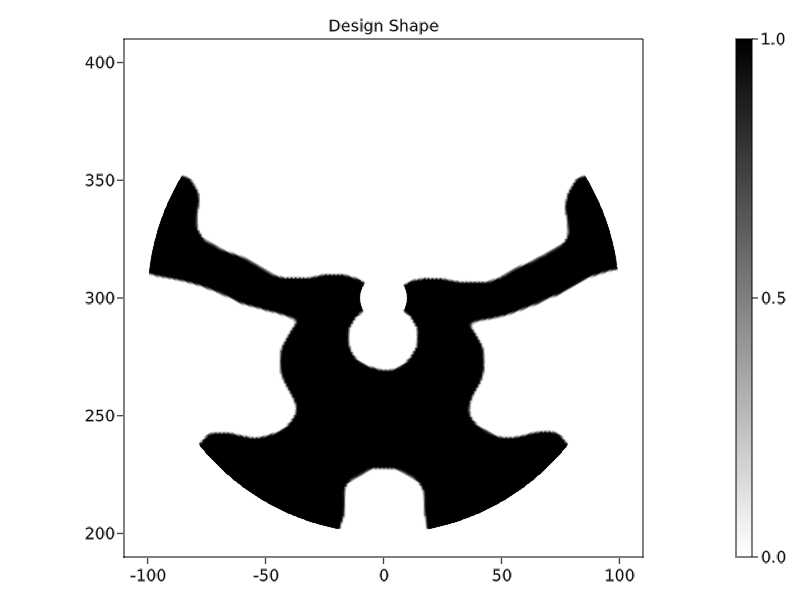

For the electric field, recall that $\vert E\vert^2\sim\vert \frac{1}{\epsilon}\nabla H\vert^2$, the factor 2 below comes from the amplitude compared to the incident plane wave. We can see that the optimized shapes are very similar to the optimized shape in Ref. [6], proving our results.

maxe = 30 # Maximum electric field magnitude compared to the incident plane wave
e1=abs2(phys_params.n_air^2)
e2=abs2(phys_params.n_metal^2)

fig, ax, plt = plot(fem_params.Ω, 2*(sqrt∘(abs((conj(∇(uh)) ⋅ ∇(uh))/(CellField(e1,fem_params.Ω) + (e2 - e1) * pth)))), colormap = :hot, colorrange=(0, maxe))
Colorbar(fig[1,2], plt)
ax.title = "|E|"
ax.aspect = AxisAspect(1)
limits!(ax, -rplot, rplot, (h1)/2-rplot, (h1)/2+rplot)
save("Field.png", fig)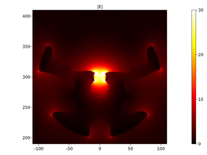

References

[1] Wikipedia: Electromagnetic wave equation

[2] Wikipedia: Perfectly matched layer

[3] A. Oskooi and S. G. Johnson, “Distinguishing correct from incorrect PML proposals and a corrected unsplit PML for anisotropic, dispersive media,” Journal of Computational Physics, vol. 230, pp. 2369–2377, April 2011.

[4] R. E. Christiansen, J. Vester-Petersen, S.P. Madsen, and O. Sigmund, “A non-linear material interpolation for design of metallic nano-particles using topology optimization,” Computer Methods in Applied Mechanics and Engineering , vol. 343, pp. 23–39, January 2019.

[5] B. S. Lazarov and O. Sigmund, "Filters in topology optimization based on Helmholtz-type differential equations", International Journal for Numerical Methods in Engineering, vol. 86, pp. 765-781, December 2010.

[6] R.E. Christiansen, J. Michon, M. Benzaouia, O. Sigmund, and S.G. Johnson, "Inverse design of nanoparticles for enhanced Raman scattering," Optical Express, vol. 28, pp. 4444-4462, February 2020.

This page was generated using Literate.jl.