Tutorial 6: Poisson equation (with DG)

In this tutorial, we will learn

How to solve a simple PDE with a DG method
How to compute jumps and averages of quantities on the mesh skeleton
How to implement the method of manufactured solutions
How to integrate error norms
How to generate Cartesian meshes in arbitrary dimensions

Problem statement

The goal of this tutorial is to solve a PDE using a Discontinuous Galerkin (DG) formulation. For simplicity, we take the Poisson equation on the unit cube $\Omega \doteq (0,1)^3$ as the model problem, namely

\[\left\lbrace \begin{aligned} -\Delta u = f \ &\text{in} \ \Omega,\\ u = g \ &\text{on}\ \Gamma \doteq \partial\Omega,\\ \end{aligned} \right.\]

where $f$ is the source term and $g$ is the prescribed Dirichlet boundary function. In this tutorial, we follow the method of manufactured solutions since we want to illustrate how to compute discretization errors. We take $u(x) = 3 x_1 + x_2^2 + 2 x_3^3 + x_1 x_2 x_3 $ as the exact solution of the problem, for which $f(x)= -2 - 12x_3 $ and $g(x) = u(x)$. The selected manufactured solution $u$ is a third order multi-variate polynomial, which can be represented exactly by the FE discretization that we are going to define below. In this scenario, the discretization error has to be close to the machine precision. We will use this result to validate the proposed implementation.

Numerical Scheme

We consider a DG formulation to approximate the problem. In particular, we consider the symmetric interior penalty method (see, e.g. [1], for specific details). For this formulation, the approximation space is made of discontinuous piece-wise polynomials, namely

\[V \doteq \{ v\in L^2(\Omega):\ v|_{T}\in Q_p(T) \text{ for all } T\in\mathcal{T} \},\]

where $\mathcal{T}$ is the set of all cells $T$ of the FE mesh, and $Q_p(T)$ is a polynomial space of degree $p$ defined on a generic cell $T$. For simplicity, we consider Cartesian meshes in this tutorial. In this case, the space $Q_p(T)$ is made of multi-variate polynomials up to degree $p$ in each spatial coordinate.

In order to write the weak form of the problem, we need to introduce some notation. The sets of interior and boundary facets associated with the FE mesh $\mathcal{T}$ are denoted here as $\mathcal{F}_\Lambda$ and $\mathcal{F}_{\Gamma}$ respectively. In addition, for a given function $v\in V$ restricted to the interior facets $\mathcal{F}_\Lambda$, we introduce the well known jump and mean value operators,

\[\begin{aligned} \lbrack\!\lbrack v\ n \rbrack\!\rbrack &\doteq v^+\ n^+ + v^- n^-,\\ \{\! \!\{\nabla v\}\! \!\} &\doteq \dfrac{ \nabla v^+ + \nabla v^-}{2}, \end{aligned}\]

with $v^+$, and $v^-$ being the restrictions of $v\in V$ to the cells $T^+$, $T^-$ that share a generic interior facet in $\mathcal{F}_\Lambda$, and $n^+$, and $n^-$ are the facet outward unit normals from either the perspective of $T^+$ and $T^-$ respectively.

With this notation, the weak form associated with the interior penalty formulation of our problem reads: find $u\in V$ such that $a(u,v) = l(v)$ for all $v\in V$. The bilinear and linear forms $a(\cdot,\cdot)$ and $l(\cdot)$ have contributions associated with the bulk of $\Omega$, the boundary facets $\mathcal{F}_{\Gamma}$, and the interior facets $\mathcal{F}_\Lambda$, namely

\[\begin{aligned} a(u,v) &= a_{\Omega}(u,v) + a_{\Gamma}(u,v) + a_{\Lambda}(u,v),\\ l(v) &= l_{\Omega}(v) + l_{\Gamma}(v). \end{aligned}\]

These contributions are defined as

\[\begin{aligned} a_{\Omega}(u,v) &\doteq \sum_{T\in\mathcal{T}} \int_{T} \nabla v \cdot \nabla u \ {\rm d}T, \\ l_{\Omega}(v) &\doteq \int_{\Omega} v\ f \ {\rm d}\Omega, \end{aligned}\]

for the volume,

\[\begin{aligned} a_{\Gamma}(u,v) \doteq & - \sum_{F\in\mathcal{F}_{\Gamma}} \int_{F} v\ (\nabla u \cdot n) \ {\rm d}F \\ & - \sum_{F\in\mathcal{F}_{\Gamma}} \int_{F} (\nabla v \cdot n)\ u \ {\rm d}F \\ & + \sum_{F\in\mathcal{F}_{\Gamma}} \dfrac{\gamma}{|F|} \int_{F} v\ u \ {\rm d}F, \\ l_{\Gamma}(v) \doteq & - \sum_{F\in\mathcal{F}_{\Gamma}} \int_{F} (\nabla v \cdot n)\ g \ {\rm d}F \\ & + \sum_{F\in\mathcal{F}_{\Gamma}} \dfrac{\gamma}{|F|} \int_{F} v\ g \ {\rm d}F, \end{aligned}\]

for the boundary facets and,

\[\begin{aligned} a_{\Lambda}(u,v) \doteq & - \sum_{F\in\mathcal{F}_{\Lambda}} \int_{F} \lbrack\!\lbrack v\ n \rbrack\!\rbrack\cdot \{\! \!\{\nabla u\}\! \!\} \ {\rm d}F \\ & - \sum_{F\in\mathcal{F}_{\Lambda}} \int_{F} \{\! \!\{\nabla v\}\! \!\}\cdot \lbrack\!\lbrack u\ n \rbrack\!\rbrack \ {\rm d}F \\ & + \sum_{F\in\mathcal{F}_{\Lambda}} \dfrac{\gamma}{|F|} \int_{F} \lbrack\!\lbrack v\ n \rbrack\!\rbrack\cdot \lbrack\!\lbrack u\ n \rbrack\!\rbrack \ {\rm d}F, \end{aligned}\]

for the interior facets. In previous expressions, $|F|$ denotes the diameter of the face $F$ (in our Cartesian grid, this is equivalent to the characteristic mesh size $h$), and $\gamma$ is a stabilization parameter that should be chosen large enough such that the bilinear form $a(\cdot,\cdot)$ is stable and continuous. Here, we take $\gamma = p\ (p+1)$ as done in the numerical experiments in reference [2].

Manufactured solution

We start by loading the Gridap library and defining the manufactured solution $u$ and the associated source term $f$ and Dirichlet function $g$.

using Gridap
u(x) = 3*x[1] + x[2]^2 + 2*x[3]^3 + x[1]*x[2]*x[3]
f(x) = -2 - 12*x[3]
g(x) = u(x)

We also need to define the gradient of $u$ since we will compute the $H^1$ error norm later. In that case, the gradient is simply defined as

∇u(x) = VectorValue(3        + x[2]*x[3],
                    2*x[2]   + x[1]*x[3],
                    6*x[3]^2 + x[1]*x[2])

In addition, we need to tell the Gridap library that the gradient of the function u is available in the function ∇u (at this moment u and ∇u are two standard Julia functions without any connection between them). This is done by adding an extra method to the function gradient (aka ∇) defined in Gridap:

import Gridap: ∇
∇(::typeof(u)) = ∇u

Now, it is possible to recover function ∇u from function u as ∇(u). You can check that the following expression evaluates to true.

∇(u) === ∇u

Cartesian mesh generation

In order to discretize the geometry of the unit cube, we use the Cartesian mesh generator available in Gridap.

L = 1.0
domain = (0.0, L, 0.0, L, 0.0, L)
n = 4
partition = (n,n,n)
model = CartesianDiscreteModel(domain,partition)

The type CartesianDiscreteModel is a concrete type that inherits from DiscreteModel, which is specifically designed for building Cartesian meshes. The CartesianDiscreteModel constructor takes a tuple containing limits of the box we want to discretize plus a tuple with the number of cells to be generated in each direction (here $4\times4\times4$ cells). You can write the model in vtk format to visualize it (see next figure).

 writevtk(model,"model")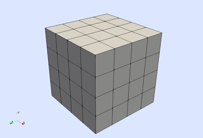

Note that the CaresianDiscreteModel is implemented for arbitrary dimensions. For instance, the following lines build a CartesianDiscreteModel for the unit square $(0,1)^2$ with 4 cells per direction

domain2D = (0.0, L, 0.0, L)
partition2D = (n,n)
model2D = CartesianDiscreteModel(domain2D,partition2D)

You could also generate a mesh for the unit tesseract $(0,1)^4$ (i.e., the unit cube in 4D). Look how the 2D and 3D models are built and just follow the sequence.

FE spaces

On top of the discrete model, we create the discontinuous space $V$ as follows

order = 3
V = TestFESpace(model,
                ReferenceFE(lagrangian,Float64,order),
                conformity=:L2)

We have select a Lagrangian, scalar-valued interpolation of order $3$ within the cells of the discrete model. Since the cells are hexahedra, the resulting Lagrangian shape functions are tri-cubic polynomials. In contrast to previous tutorials, where we have constructed $H^1$-conforming (i.e., continuous) FE spaces, here we construct a $L^2$-conforming (i.e., discontinuous) FE space. That is, we do not impose any type of continuity of the shape function on the cell boundaries, which leads to the discontinuous FE space $V$ of the DG formulation. Note also that we do not pass any information about the Dirichlet boundary to the TestFESpace constructor since the Dirichlet boundary conditions are not imposed strongly in this example.

From the V object we have constructed in previous code snippet, we build the trial FE space as usual.

U = TrialFESpace(V)

Note that we do not pass any Dirichlet function to the TrialFESpace constructor since we do not impose Dirichlet boundary conditions strongly here.

Numerical integration

Once the FE spaces are ready, the next step is to set up the numerical integration. In this example, we need to integrate in three different domains: the volume covered by the cells $\mathcal{T}$ (i.e., the computational domain $\Omega$), the surface covered by the boundary facets $\mathcal{F}_{\Gamma}$ (i.e., the boundary $\Gamma = \partial \Omega$), and the surface covered by the interior facets $\mathcal{F}_{\Lambda}$ (i.e. the so-called mesh skeleton). In order to integrate in $\Omega$ and on its boundary $\Gamma$, we use Triangulation and BoundaryTriangulation objects as already discussed in previous tutorials.

Ω = Triangulation(model)
Γ = BoundaryTriangulation(model)

Here, we do not pass any boundary identifier to the BoundaryTriangulation constructor. In this case, an integration mesh for the entire boundary $\Gamma$ is constructed by default (which is just what we need in this example).

In order to generate an integration mesh for the interior facets $\mathcal{F}_{\Lambda}$, we use a new type of Triangulation referred to as SkeletonTriangulation. It can be constructed from a DiscreteModel object as follows:

Λ = SkeletonTriangulation(model)

As any other type of Triangulation, an SkeletonTriangulation can be written into a vtk file for its visualization (see next figure, where the interior facets $\mathcal{F}_\Lambda$ are clearly observed).

writevtk(Λ,"strian")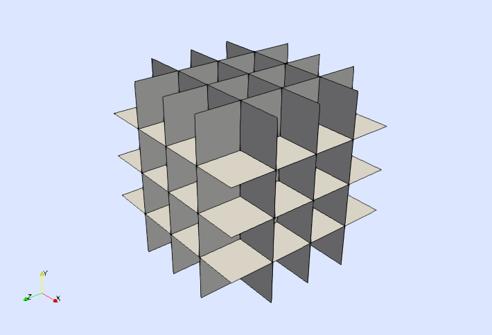

Once we have constructed the triangulations needed in this example, we define the corresponding quadrature rules by passing the triangulations together with the desired degree to the Measure function.

degree = 2*order

dΩ = Measure(Ω,degree)
dΓ = Measure(Γ,degree)
dΛ = Measure(Λ,degree)

We still need a way to represent the unit outward normal vector to the boundary $\Gamma$, and the unit normal vector on the interior faces $\mathcal{F}_\Lambda$. This is done with the get_normal_vector getter.

n_Γ = get_normal_vector(Γ)
n_Λ = get_normal_vector(Λ)

The get_normal_vector getter takes either a boundary or a skeleton triangulation and returns an object representing the normal vector to the corresponding surface. For boundary triangulations, the returned normal vector is the unit outwards one, whereas for skeleton triangulations the orientation of the returned normal is arbitrary. In the current implementation (Gridap v0.5.0), the unit normal is outwards to the cell with smaller id among the two cells that share an interior facet in $\mathcal{F}_\Lambda$.

Weak form

With these ingredients we can define the different terms in the weak form. First, we start with the terms $a_\Omega(\cdot,\cdot)$ , and $l_\Omega(\cdot)$ associated with integrals in the volume $\Omega$. This is done as in the tutorial for the Poisson equation.

a_Ω(u,v) = ∫( ∇(v)⊙∇(u) )dΩ
l_Ω(v) = ∫( v*f )dΩ

The terms $a_{\Gamma}(\cdot,\cdot)$ and $l_{\Gamma}(\cdot)$ associated with integrals on the boundary $\Gamma$ are defined using an analogous approach:

h = L / n
γ = order*(order+1)
a_Γ(u,v) = ∫( - v*(∇(u)⋅n_Γ) - (∇(v)⋅n_Γ)*u + (γ/h)*v*u )dΓ
l_Γ(v)   = ∫(                - (∇(v)⋅n_Γ)*g + (γ/h)*v*g )dΓ

Note that in the definition of the functions a_Γ and b_Γ, we have used the object n_Γ representing the outward unit normal to the boundary $\Gamma$. The code definition of a_Γ and b_Γ is indeed very close to the mathematical definition of the forms $a_{\Gamma}(\cdot,\cdot)$ and $b_{\Gamma}(\cdot)$.

Finally, we need to define the term $a_\Lambda(\cdot,\cdot)$ integrated on the interior facets $\mathcal{F}_\Lambda$,

a_Λ(u,v) = ∫( - jump(v*n_Λ)⊙mean(∇(u))
              - mean(∇(v))⊙jump(u*n_Λ)
              + (γ/h)*jump(v*n_Λ)⊙jump(u*n_Λ) )dΛ

Note that the arguments v, u of function a_Λ represent a test and trial function restricted to the interior facets $\mathcal{F}_\Lambda$. As mentioned before in the presentation of the DG formulation, the restriction of a function $v\in V$ to the interior faces leads to two different values $v^+$ and $v^-$ . In order to compute jumps and averages of the quantities $v^+$ and $v^-$, we use the functions jump and mean, which represent the jump and mean value operators $\lbrack\!\lbrack \cdot \rbrack\!\rbrack$ and $\{\! \!\{\cdot\}\! \!\}$ respectively. Note also that we have used the object n_Λ representing the unit normal vector on the interior facets. As a result, the notation used to define function a_Λ is very close to the mathematical definition of the terms in the bilinear form $a_\Lambda(\cdot,\cdot)$.

Once the different terms of the weak form have been defined, we build and solve the FE problem.

a(u,v) = a_Ω(u,v) + a_Γ(u,v) + a_Λ(u,v)
l(v) = l_Ω(v) + l_Γ(v)

op = AffineFEOperator(a, l, U, V)
uh = solve(op)

Discretization error

We end this tutorial by quantifying the discretization error associated with the computed numerical solution uh. In DG methods a simple error indicator is the jump of the computed (discontinuous) approximation on the interior faces. We compute and visualize the jump of these values as follows (see next figure):

writevtk(Λ,"jumps",cellfields=["jump_u"=>jump(uh)])

Note that the jump of the numerical solution is very small, close to the machine precision (as expected in this example with manufactured solution).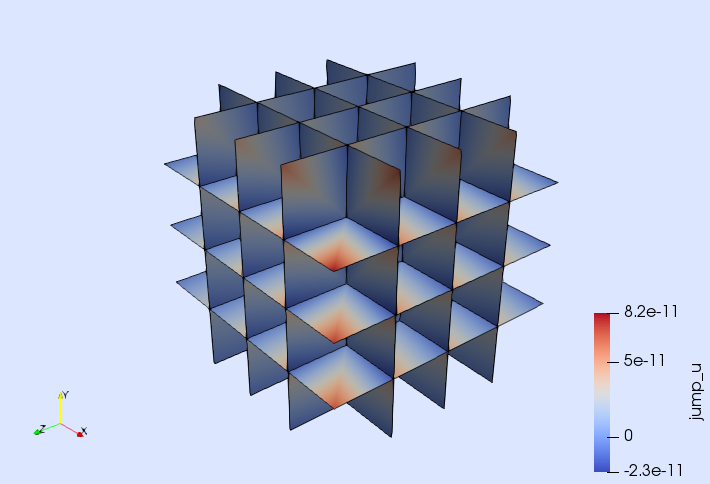

A more rigorous way of quantifying the error is to measure it with a norm. Here, we use the $L^2$ and $H^1$ norms, namely

\[\begin{aligned} \| w \|_{L^2}^2 & \doteq \int_{\Omega} w^2 \ \text{d}\Omega, \\ \| w \|_{H^1}^2 & \doteq \int_{\Omega} w^2 + \nabla w \cdot \nabla w \ \text{d}\Omega. \end{aligned}\]

The discretization error can be computed in this example as the difference of the manufactured and numerical solutions.

e = u - uh

We compute the error norms as follows. First, we implement the integrands of the norms we want to compute.

l2(u) = sqrt(sum( ∫( u⊙u )*dΩ ))
h1(u) = sqrt(sum( ∫( u⊙u + ∇(u)⊙∇(u) )*dΩ ))

Then, we compute the corresponding integrals with the integrate function.

el2 = l2(e)
eh1 = h1(e)

The integrate function returns a lazy object representing the contribution to the integral of each cell in the underlying triangulation. To end up with the desired error norms, one has to sum these contributions and take the square root. You can check that the computed error norms are close to machine precision (as one would expect).

tol = 1.e-10
@assert el2 < tol
@assert eh1 < tol

References

[1] D. N. Arnold, F. Brezzi, B. Cockburn, and L. Donatella Marini. Unified analysis of discontinuous Galerkin methods for elliptic problems. SIAM Journal on Numerical Analysis, 39 (5):1749–1779, 2001. doi:10.1137/S0036142901384162.

[2] B. Cockburn, G. Kanschat, and D. Schötzau. An equal-order DG method for the incompressible Navier-Stokes equations. Journal of Scientific Computing, 40(1-3):188–210, 2009. doi:10.1007/s10915-008-9261-1.

This page was generated using Literate.jl.