Tutorial 3: Linear elasticity

In this tutorial, we will learn

• How to approximate vector-valued problems
• How to solve problems with complex constitutive laws
• How to impose Dirichlet boundary conditions only in selected components
• How to impose Dirichlet boundary conditions described by more than one function

Problem statement

In this tutorial, we detail how to solve a linear elasticity problem defined on the 3D domain depicted in next figure.

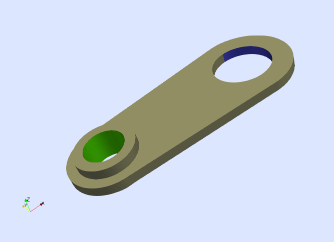
We impose the following boundary conditions. All components of the displacement vector are constrained to zero on the surface $\Gamma_{\rm G}$, which is marked in green in the figure. On the other hand, the first component of the displacement vector is prescribed to the value $\delta\doteq 5$mm on the surface $\Gamma_{\rm B}$, which is marked in blue. No body or surface forces are included in this example. Formally, the PDE to solve is

The variable $u$ stands for the unknown displacement vector, the vector $n$ is the unit outward normal to the Neumann boundary $\Gamma_{\rm N}\doteq\partial\Omega\setminus\left(\Gamma_{\rm B}\cup\Gamma_{\rm G}\right)$ and $\sigma(u)$ is the stress tensor defined as

where $I$ is the 2nd order identity tensor, and $\lambda$ and $\mu$ are the Lamé parameters of the material. The operator $\varepsilon(u)\doteq\frac{1}{2}\left(\nabla u + (\nabla u)^t \right)$ is the symmetric gradient operator (i.e., the strain tensor). Here, we consider material parameters corresponding to aluminum with Young's modulus $E=70\cdot 10^9$ Pa and Poisson's ratio $\nu=0.33$. From these values, the Lamé parameters are obtained as $\lambda = (E\nu)/((1+\nu)(1-2\nu))$ and $\mu=E/(2(1+\nu))$.

Numerical scheme

As in previous tutorial, we use a conventional Galerkin FE method with conforming Lagrangian FE spaces. For this formulation, the weak form is: find $u\in U$ such that $ a(u,v) = 0 $ for all $v\in V_0$, where $U$ is the subset of functions in $V\doteq[H^1(\Omega)]^3$ that fulfill the Dirichlet boundary conditions of the problem, whereas $V_0$ are functions in $V$ fulfilling $v=0$ on $\Gamma_{\rm G}$ and $v_1=0$ on $\Gamma_{\rm B}$. The bilinear form of the problem is

The main differences with respect to previous tutorial is that we need to deal with a vector-valued problem, we need to impose different prescribed values on the Dirichlet boundary, and the integrand of the bilinear form $a(\cdot,\cdot)$ is more complex as it involves the symmetric gradient operator and the stress tensor. However, the implementation of this numerical scheme is still done in a user-friendly way since all these features can be easily accounted for with the abstractions in the library.

Discrete model

We start by loading the discrete model from a file

using Gridap
model = DiscreteModelFromFile("../models/solid.json")

In order to inspect it, write the model to vtk

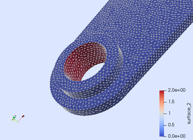
writevtk(model,"model")

and open the resulting files with Paraview. The boundaries $\Gamma_{\rm B}$ and $\Gamma_{\rm G}$ are identified with the names "surface_1" and "surface_2" respectively. For instance, if you visualize the faces of the model and color them by the field "surface_2" (see next figure), you will see that only the faces on $\Gamma_{\rm G}$ have a value different from zero.

Vector-valued FE space

The next step is the construction of the FE space. Here, we need to build a vector-valued FE space, which is done as follows:

order = 1

reffe = ReferenceFE(lagrangian,VectorValue{3,Float64},order)
V0 = TestFESpace(model,reffe;
  conformity=:H1,
  dirichlet_tags=["surface_1","surface_2"],
  dirichlet_masks=[(true,false,false), (true,true,true)])

As in previous tutorial, we construct a continuous Lagrangian interpolation of order 1. The vector-valued interpolation is selected via the option valuetype=VectorValue{3,Float64}, where we use the type VectorValue{3,Float64}, which is the way Gridap represents vectors of three Float64 components. We mark as Dirichlet the objects identified with the tags "surface_1" and "surface_2" using the dirichlet_tags argument. Finally, we chose which components of the displacement are actually constrained on the Dirichlet boundary via the dirichlet_masks argument. Note that we constrain only the first component on the boundary $\Gamma_{\rm B}$ (identified as "surface_1"), whereas we constrain all components on $\Gamma_{\rm G}$ (identified as "surface_2").

The construction of the trial space is slightly different in this case. The Dirichlet boundary conditions are described with two different functions, one for boundary $\Gamma_{\rm B}$ and another one for $\Gamma_{\rm G}$. These functions can be defined as

g1(x) = VectorValue(0.005,0.0,0.0)
g2(x) = VectorValue(0.0,0.0,0.0)

From functions g1 and g2, we define the trial space as follows:

U = TrialFESpace(V0,[g1,g2])

Note that the functions g1 and g2 are passed to the TrialFESpace constructor in the same order as the boundary identifiers are passed previously in the dirichlet_tags argument of the TestFESpace constructor.

Constitutive law

Once the FE spaces are defined, the next step is to define the weak form. In this example, the construction of the weak form requires more work than in previous tutorial since we need to account for the constitutive law that relates strain and stress. The symmetric gradient operator is represented by the function ε provided by Gridap (also available as symmetric_gradient). However, function σ representing the stress tensor is not predefined in the library and it has to be defined ad-hoc by the user, namely

const E = 70.0e9
const ν = 0.33
const λ = (E*ν)/((1+ν)*(1-2*ν))
const μ = E/(2*(1+ν))
σ(ε) = λ*tr(ε)*one(ε) + 2*μ*ε

Function σ takes a strain tensor ε(one can interpret this strain as the strain at an arbitrary integration point) and computes the associated stress tensor using the Lamé operator. Note that the implementation of function σ is very close to its mathematical definition.

Weak form

As seen in previous tutorials, in order to define the weak form we need to build the integration mesh and the corresponding measure

degree = 2*order
Ω = Triangulation(model)
dΩ = Measure(Ω,degree)

From these objects and the constitutive law previously defined, we can write the weak form as follows

a(u,v) = ∫( ε(v) ⊙ (σ∘ε(u)) )*dΩ
l(v) = 0

Note that we have composed function σ with the strain field ε(u) in order to compute the stress field associated with the trial function u. The linear form is simply l(v) = 0 since there are not external forces in this example.

Solution of the FE problem

The remaining steps for solving the FE problem are essentially the same as in previous tutorial.

op = AffineFEOperator(a,l,U,V0)
uh = solve(op)

Note that we do not have explicitly constructed a LinearFESolver in order to solve the FE problem. If a LinearFESolver is not passed to the solve function, a default solver (LU factorization) is created and used internally.

Finally, we write the results to a file. Note that we also include the strain and stress tensors into the results file.

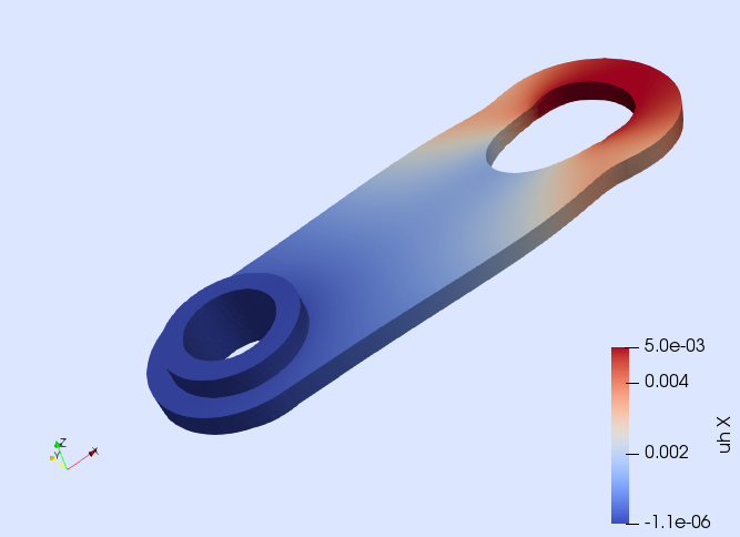
writevtk(Ω,"results",cellfields=["uh"=>uh,"epsi"=>ε(uh),"sigma"=>σ∘ε(uh)])

It can be clearly observed (see next figure) that the surface $\Gamma_{\rm B}$ is pulled in $x_1$-direction and that the solid deforms accordingly.

Multi-material problems

We end this tutorial by extending previous code to deal with multi-material problems. Let us assume that the piece simulated before is now made of 2 different materials (see next figure). In particular, we assume that the volume depicted in dark green is made of aluminum, whereas the volume marked in purple is made of steel.

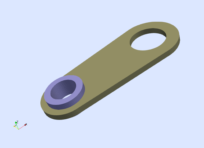
The two different material volumes are properly identified in the model we have previously loaded. To check this, inspect the model with Paraview (by writing it to vtk format as done before). Note that the volume made of aluminum is identified as "material_1", whereas the volume made of steel is identified as "material_2".

In order to build the constitutive law for the bi-material problem, we need a vector that contains information about the material each cell in the model is composed. This is achieved by these lines

using Gridap.Geometry
labels = get_face_labeling(model)
dimension = 3
tags = get_face_tag(labels,dimension)

Previous lines generate a vector, namely tags, whose length is the number of cells in the model and for each cell contains an integer that identifies the material of the cell. This is almost what we need. We also need to know which is the integer value associated with each material. E.g., the integer value associated with "material_1" (i.e. aluminum) is retrieved as

const alu_tag = get_tag_from_name(labels,"material_1")

Now, we know that cells whose corresponding value in the tags vector is alu_tag are made of aluminum, otherwise they are made of steel (since there are only two materials in this example).

At this point, we are ready to define the multi-material constitutive law. First, we define the material parameters for aluminum and steel respectively:

function lame_parameters(E,ν)
  λ = (E*ν)/((1+ν)*(1-2*ν))
  μ = E/(2*(1+ν))
  (λ, μ)
end

const E_alu = 70.0e9
const ν_alu = 0.33
const (λ_alu,μ_alu) = lame_parameters(E_alu,ν_alu)

const E_steel = 200.0e9
const ν_steel = 0.33
const (λ_steel,μ_steel) = lame_parameters(E_steel,ν_steel)

Then, we define the function containing the constitutive law:

function σ_bimat(ε,tag)
  if tag == alu_tag
    return λ_alu*tr(ε)*one(ε) + 2*μ_alu*ε
  else
    return λ_steel*tr(ε)*one(ε) + 2*μ_steel*ε
  end
end

Note that in this new version of the constitutive law, we have included a third argument that represents the integer value associated with a certain material. If the value corresponds to the one for aluminum (i.e., tag == alu_tag), then, we use the constitutive law for this material, otherwise, we use the law for steel.

Since we have constructed a new constitutive law, we need to re-define the bilinear form of the problem:

a(u,v) = ∫( ε(v) ⊙ (σ_bimat∘(ε(u),tags)) )*dΩ

In previous line, pay attention in the usage of the new constitutive law σ_bimat. Note that we have passed the vector tags containing the material identifiers in the last argument of the function`.

At this point, we can build the FE problem again and solve it

op = AffineFEOperator(a,l,U,V0)
uh = solve(op)

Once the solution is computed, we can store the results in a file for visualization. Note that, we are including the stress tensor in the file (computed with the bi-material law).

writevtk(Ω,"results_bimat",cellfields=
  ["uh"=>uh,"epsi"=>ε(uh),"sigma"=>σ_bimat∘(ε(uh),tags)])

Tutorial done!

This page was generated using Literate.jl.