Tutorial 1: Parameterised PDEs

In this tutorial we learn how to

• define a space of parameters and sample it
• write parameter-dependent data, FE spaces and weak forms
• build and solve parameterised FE problems, steady and transient

No reduced order model appears here: this is the high-fidelity layer that every ROM in GridapROMs is built upon. If you are new to Gridap, have a look at its tutorials first — GridapROMs follows the same API, and only adds the parameter μ on top.

Problem statement

We consider a Poisson problem on the unit square $\Omega = (0,1)^2$, parameterised by $\mu = (\mu_1,\mu_2,\mu_3) \in \mathcal{D} = [1,10]^3$:

\[\left\{ \begin{aligned} -\nabla \cdot (\kappa_\mu \nabla u_\mu) &= f & \text{in } \Omega, \\ u_\mu &= g_\mu & \text{on } \Gamma_D, \\ \kappa_\mu \nabla u_\mu \cdot n &= h_\mu & \text{on } \Gamma_N, \end{aligned} \right.\]

where $\Gamma_D$ is the union of the left and bottom edges of the square, and $\Gamma_N$ the top edge (a homogeneous Neumann condition holds on the right edge). The data are

\[\kappa_\mu(x) = 1 + \mu_1 e^{-x_1 x_2}, \qquad f(x) = 10, \qquad g_\mu(x) = e^{-x_1/\mu_2}, \qquad h_\mu(x) = 5\cos(\mu_3 x_1).\]

For every $\mu \in \mathcal{D}$ we obtain a different solution $u_\mu$. Solving many such problems is exactly the many-query scenario that ROMs target.

using Gridap
using GridapROMs
using Plots

Plots.GRBackend()

The parameter space

A ParamSpace is defined by the bounds of each parameter component:

pdomain = (1,10,1,10,1,10)
D = ParamSpace(pdomain)

Set of parameters in [[1, 10], [1, 10], [1, 10]], sampled with HaltonSampling(1)

A Realisation is a collection of parameters sampled from D. By default, samples follow a Halton sequence:

μ = realisation(D;nparams=3)

Realisation{Vector{Vector{Float64}}}([[5.5, 4.0, 2.8], [3.25, 7.0, 4.6], [7.75, 2.0, 6.4]])

Other sampling strategies are available through the keyword sampling (:halton, :uniform, :normal, :latin_hypercube, :tensorial_uniform):

μ_unif = realisation(D;nparams=3,sampling=:uniform)

Realisation{Vector{Vector{Float64}}}([[7.892577603963795, 7.015675535597493, 3.7799307789264036], [2.146414972148758, 3.6216222294035365, 8.136082491742261], [7.5326235239487325, 6.741860633481805, 2.7522745238995108]])

Parameterised data

A parameter-dependent function is written as a function of μ returning a function of space x. The function parameterise turns it into a ParamFunction, which can be evaluated for a whole realisation at once:

κ(μ) = x -> 1 + μ[1]*exp(-x[1]*x[2])
κμ(μ) = parameterise(κ,μ)

g(μ) = x -> exp(-x[1]/μ[2])
gμ(μ) = parameterise(g,μ)

h(μ) = x -> 5*cos(μ[3]*x[1])
hμ(μ) = parameterise(h,μ)

f(x) = 10.0

f (generic function with 1 method)

Parameter-independent data (like f) are plain Julia functions, as in Gridap.

Geometry and FE spaces

The geometry and the test space are exactly as in Gridap. The trial space is a ParamTrialFESpace, which takes a parameterised Dirichlet datum:

model = CartesianDiscreteModel((0,1,0,1),(40,40))

order = 1
reffe = ReferenceFE(lagrangian,Float64,order)
V = TestFESpace(model,reffe;conformity=:H1,dirichlet_tags=[1,2,3,5,7])
U = ParamTrialFESpace(V,gμ)

UnEvalTrialFESpace()

The tags [1,2,3,5,7] select the left and bottom edges, including their end points. U is not a FE space yet: it becomes one once evaluated at a realisation, e.g. U(μ), which is a single FE space whose Dirichlet values are stored for all the parameters in μ.

Weak form

The weak forms take the parameter as first argument. The Neumann boundary is the top edge of the square (tag 6):

Ω = Triangulation(model)
Γn = BoundaryTriangulation(model;tags=6)

degree = 2*order
dΩ = Measure(Ω,degree)
dΓn = Measure(Γn,degree)

a(μ,u,v) = ∫(κμ(μ)*∇(v)⋅∇(u))dΩ
l(μ,v) = ∫(f*v)dΩ + ∫(hμ(μ)*v)dΓn

l (generic function with 1 method)

The parameterised operator

Since the problem is linear in u, we build a LinearParamOperator from the right-hand side l, the bilinear form a, the parameter space, and the FE spaces:

feop = LinearParamOperator(l,a,D,U,V)

GenericParamOperator()

Nonlinear problems are defined with a ParamOperator, given a residual res(μ,u,v) and a Jacobian jac(μ,u,du,v), as in Gridap's FEOperator.

Solving

Any Gridap linear (or nonlinear) solver can be used. A single call solves the problem for all the parameters in a realisation:

solver = LUSolver()
u = solve(solver,feop,μ)

3-element GridapROMs.ParamDataStructures.ConsecutiveParamVector{Float64, Matrix{Float64}}:
 [0.996518767924857, 0.9925054358896042, 0.988227983253318, 0.983779607695107, 0.9792095138773957, 0.9745477656770903, 0.9698145862836859, 0.9650244890814388, 0.9601884010426565, 0.9553148642120827  …  1.2125796344022548, 1.1978130025339242, 1.1835464748816482, 1.1700083538978192, 1.1574421665963588, 1.146113113772937, 1.1363199192523772, 1.1284194878742093, 1.1228795582421218, 1.1205977827029951]
 [1.0001908953454586, 0.9995515806940684, 0.9984801354321624, 0.9971155300447683, 0.9955314985279913, 0.9937733740663605, 0.991871869776437, 0.9898491963015772, 0.9877222032407551, 0.9855041537077865  …  1.091983349994432, 1.1035287275932124, 1.117629058012667, 1.133823624025677, 1.1515076611611783, 1.169905360837521, 1.1880229790592884, 1.204553045411626, 1.2176703973112473, 1.22377687405505]
 [0.9900293538973597, 0.9797132705900387, 0.9692841061310756, 0.9588221515216027, 0.9483694177403938, 0.937951251584794, 0.927584420816297, 0.9172807022955504, 0.9070487240877184, 0.8968950061811913  …  1.324982889056729, 1.354948679534414, 1.3836147448333358, 1.4102928066606673, 1.4343129519509767, 1.455042424934975, 1.4719042214357092, 1.4843951031247227, 1.492102803543774, 1.4947236647467401]

The output u is a parameterised vector of free DOF values: one vector per parameter, stored contiguously.

param_length(u)

3

To post-process, we build a FE function in U(μ) and extract the component relative to the i-th parameter with param_getindex:

uh = FEFunction(U(μ),u)
uh1 = param_getindex(uh,1)

SingleFieldFEFunction():
 num_cells: 1600
 DomainStyle: Gridap.CellData.ReferenceDomain()
 Triangulation: BodyFittedTriangulation()
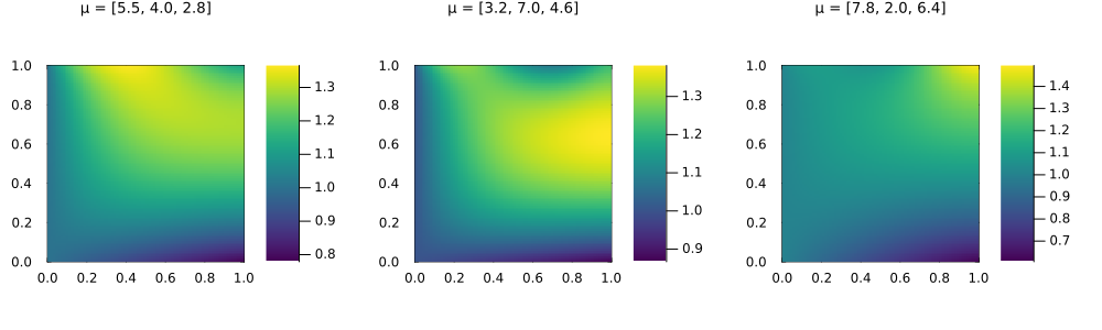
 Triangulation id: 16119849743471976209

This is a standard Gridap FE function: it can be integrated, evaluated, or written to VTK with writevtk. Here we plot the three solutions with a small helper:

function plot_field(uh;n=101,kwargs...)
  xs = range(0,1;length=n)
  pts = [Point(x,y) for x in xs, y in xs]
  vals = reshape(uh(vec(pts)),n,n)
  heatmap(xs,xs,permutedims(vals);aspect_ratio=:equal,framestyle=:box,
    xlims=(0,1),ylims=(0,1),c=:viridis,kwargs...)
end

plts = map(enumerate(μ)) do (i,μi)
  plot_field(param_getindex(uh,i);title="μ = $(round.(μi;digits=1))",titlefontsize=9)
end
plot(plts...;layout=(1,3),size=(1000,300))

Snapshots

ROMs are trained on a collection of FE solutions, the snapshots. The function solution_snapshots solves the problem and wraps the result in a Snapshots structure, which also stores the realisation and the DOF ordering:

μ_train = realisation(feop;nparams=20)
snaps = solution_snapshots(solver,feop,μ_train)
size(snaps)

(1600, 20)

Snapshots behave as a matrix with one row per DOF and one column per parameter.

Transient problems

Time-dependent problems follow the same pattern. We consider the heat equation

\[\partial_t u_\mu - \nabla \cdot (\kappa_\mu \nabla u_\mu) = f \quad \text{in } \Omega \times (0,T],\]

with the same boundary conditions as before, now multiplied by $\sin(\pi t)$. Parameterised data take (μ,t) as arguments, and parameterise yields a TransientParamFunction:

gt(μ,t) = x -> exp(-x[1]/μ[2])*sin(π*t)
gμt(μ,t) = parameterise(gt,μ,t)

ht(μ,t) = x -> 5*cos(μ[3]*x[1])*sin(π*t)
hμt(μ,t) = parameterise(ht,μ,t)

κt(μ,t) = x -> 1 + μ[1]*exp(-x[1]*x[2])
κμt(μ,t) = parameterise(κt,μ,t)

κμt (generic function with 1 method)

A TransientParamSpace couples the parameter domain with a time interval. Realisations sample parameters only: the time grid is fixed by the time-marching scheme.

dt = 0.05
t0,tf = 0.0,1.0
Dt = TransientParamSpace(pdomain,t0:dt:tf)

Set of tuples (p,t) in [[1, 10], [1, 10], [1, 10]] × 0.0:0.05:1.0

The trial space is a TransientTrialParamFESpace, and the operator a TransientLinearParamOperator, built from the right-hand side and the tuple of Jacobians with respect to u (stiffness) and ∂t(u) (mass):

Ut = TransientTrialParamFESpace(V,gμt)

stiffness(μ,t,u,v) = ∫(κμt(μ,t)*∇(v)⋅∇(u))dΩ
mass(μ,t,uₜ,v) = ∫(v*uₜ)dΩ
rhs(μ,t,v) = ∫(f*v)dΩ + ∫(hμt(μ,t)*v)dΓn

feop_t = TransientLinearParamOperator(rhs,(stiffness,mass),Dt,Ut,V)

GenericParamOperator()

The time-marching scheme is any Gridap ODESolver; here, Crank–Nicolson. The initial condition is a function of μ:

θ = 0.5
fesolver_t = ThetaMethod(LUSolver(),dt,θ)

u0(μ) = x -> 0.0
u0μ(μ) = parameterise(u0,μ)
uh0μ(μ) = interpolate_everywhere(u0μ(μ),Ut(μ,t0))

μt = realisation(feop_t;nparams=2)
snaps_t = solution_snapshots(fesolver_t,feop_t,μt,uh0μ)
size(snaps_t)

(1600, 40)

Transient snapshots have one row per DOF and one column per pair (μ,t). Gridap's lazy iteration over time steps is also available, via solve(fesolver_t,feop_t,μt,uh0μ).

Summary

In the next tutorial we use these snapshots to build reduced order models.