Tutorial 3: Local reduced operators

In this tutorial we learn

• why a single (global) reduced subspace can be a poor choice
• how local reduced operators are built, stored and evaluated
• how to trade the number of clusters against the number of snapshots per cluster

Motivation

A linear ROM approximates the solution manifold $\{u_\mu\}_{\mu \in \mathcal{D}}$ with a single subspace. When the solutions change a lot across $\mathcal{D}$ (moving fronts, boundary layers, transport-dominated phenomena), the dimension of this subspace grows quickly with the required accuracy, and so does the online cost.

A local ROM partitions the parameter space into clusters, and builds a reduced operator per cluster. Each local subspace only has to approximate the solutions in its own region of $\mathcal{D}$, which requires fewer modes. Online, the parameter selects its cluster, and the corresponding (small) reduced problem is solved.

The problem

We consider an advection-diffusion problem on $\Omega = (0,1)^2$:

\[-\epsilon \Delta u + b_\mu \cdot \nabla u = 1 \ \text{in } \Omega, \qquad u = 0 \ \text{on } \partial\Omega,\]

with advection velocity $b_\mu = (\cos\mu_1, \sin\mu_1)$ and diffusion $\epsilon = \mu_2$, for $\mu \in [0,2\pi] \times [0.02,0.1]$. The boundary layer forms on the outflow side, and rotates with the advection direction:

using Gridap
using GridapROMs
using Plots

D = ParamSpace((0.0,2π,0.02,0.1))

model = CartesianDiscreteModel((0,1,0,1),(40,40))
Ω = Triangulation(model)
dΩ = Measure(Ω,2)

reffe = ReferenceFE(lagrangian,Float64,1)
V = TestFESpace(Ω,reffe;conformity=:H1,dirichlet_tags="boundary")
U = ParamTrialFESpace(V)

ϵ(μ) = x -> μ[2]
ϵμ(μ) = parameterise(ϵ,μ)
b(μ) = x -> VectorValue(cos(μ[1]),sin(μ[1]))
bμ(μ) = parameterise(b,μ)

a(μ,u,v) = ∫(ϵμ(μ)*∇(v)⋅∇(u))dΩ + ∫(v*(bμ(μ)⋅∇(u)))dΩ
l(μ,v) = ∫(v)dΩ

feop = LinearParamOperator(l,a,D,U,V,FEDomains((Ω,),(Ω,)))
solver = LUSolver()

"Gridap.Algebra.LUSolver"

Let us look at a few solutions:

function plot_field(uh;n=101,kwargs...)
  xs = range(0,1;length=n)
  pts = [Point(x,y) for x in xs, y in xs]
  vals = reshape(uh(vec(pts)),n,n)
  heatmap(xs,xs,permutedims(vals);aspect_ratio=:equal,framestyle=:box,
    xlims=(0,1),ylims=(0,1),c=:viridis,titlefontsize=10,kwargs...)
end

μ = Realisation([[0.0,0.05],[π/2,0.05],[5π/4,0.05]])
uh = FEFunction(U(μ),solve(solver,feop,μ))
plts = map(enumerate(μ)) do (i,μi)
  plot_field(param_getindex(uh,i);title="μ₁ = $(round(μi[1];digits=2))")
end
plot(plts...;layout=(1,3),size=(1000,300))

Global ROM

We first compute 100 snapshots, and the online reference solutions:

reduction = Reduction(1e-3,H1();nparams=100)
rbsolver = RBSolver(solver,reduction;nparams_res=20,nparams_jac=60,verbose=false)

fesnaps = solution_snapshots(rbsolver,feop)

μon = realisation(feop;nparams=20,sampling=:uniform)
x = solution_snapshots(rbsolver,feop,μon)

1521×20 GridapROMs.ParamDataStructures.GenericSnapshots{Float64, 2, GridapROMs.DofMaps.VectorDofMap{1, Int64, LinearIndices{1, Tuple{Base.OneTo{Int64}}}}, Realisation{Vector{Vector{Float64}}}, Matrix{Float64}, GridapROMs.ParamDataStructures.ConsecutiveParamVector{Float64, Matrix{Float64}}}:
 0.0150916  0.0168008  0.00721641  …  0.0110151  0.00922675  0.024328
 0.027482   0.0307676  0.0115145      0.019511   0.014552    0.0446579
 0.038626   0.0433322  0.0145124      0.0268908  0.0182016   0.0626329
 0.0489727  0.0549387  0.0167406      0.0335963  0.0208864   0.0788001
 0.0587338  0.0657981  0.0184618      0.0398407  0.0229478   0.0934471
 0.0680239  0.0760257  0.0198259   …  0.045744   0.0245766   0.106753
 0.0769106  0.0856907  0.0209272      0.0513806  0.0258906   0.118846
 0.0854357  0.0948377  0.0218289      0.0567998  0.0269674   0.129823
 0.0936257  0.103496   0.0225753      0.0620357  0.0278609   0.139764
 0.101498   0.111687   0.0231985      0.0671124  0.0286098   0.148738
 ⋮                                 ⋱                         
 0.029255   0.0262387  0.145392       0.0421916  0.25059     0.0234778
 0.0288859  0.0258182  0.139115       0.0418674  0.24889     0.0230167
 0.0283414  0.0252326  0.131285       0.0412641  0.244656    0.0224065
 0.0275458  0.0244157  0.121653    …  0.0402593  0.23701     0.0215914
 0.0263828  0.0232687  0.109914       0.0386666  0.224733    0.020489
 0.0246695  0.0216379  0.0956933      0.0361961  0.206128    0.0189719
 0.0221053  0.0192733  0.0785084      0.0323824  0.178807    0.0168326
 0.0181592  0.0157354  0.0577041      0.0264361  0.139356    0.0137029
 0.0117837  0.0101529  0.0322794   …  0.0168917  0.0827119   0.00883797

A global ROM with tolerance 1e-3 needs this many modes:

rbop = reduced_operator(rbsolver,feop,fesnaps)
x̂ = solution_snapshots(rbsolver,rbop,μon)
size(get_basis(rbop.trial.subspace),2), rom_performance(rbsolver,rbop,x,x̂).error

(38, 0.004506676068474251)

Local ROMs

A local ROM is obtained with the keyword compression=:local, which takes the number of clusters ncentroids:

local_reduction = Reduction(1e-3,H1();nparams=100,compression=:local,ncentroids=4)

GridapROMs.RBSteady.LocalReduction{GridapROMs.RBSteady.SearchSVDRank, H1, PODReduction{GridapROMs.RBSteady.SearchSVDRank, H1}}(PODReduction{GridapROMs.RBSteady.SearchSVDRank, H1}(GridapROMs.RBSteady.SearchSVDRank(0.001), H1(), 100), 4)

This is a LocalReduction wrapping the POD reduction. The RBSolver built from it is a LocalRBSolver, and the residual and Jacobian hyper-reductions are local as well:

local_rbsolver = RBSolver(solver,local_reduction;nparams_res=20,nparams_jac=60,verbose=false)
local_rbop = reduced_operator(local_rbsolver,feop,fesnaps)
x̂_local = solution_snapshots(local_rbsolver,local_rbop,μon)
rom_performance(local_rbsolver,local_rbop,x,x̂_local).error

0.005328721813571027

The error is similar to the global one, but the local subspaces are much smaller:

using GridapROMs.RBSteady: local_vals, get_clusters
map(p -> size(get_basis(p),2),local_vals(local_rbop.trial.subspace))

4-element Vector{Int64}:
 15
 14
 14
 16

How local operators are structured

The offline phase proceeds as follows:

1. the snapshot parameters are clustered with k-means;
2. the snapshots of each cluster are compressed separately. The resulting LocalProjection stores one projection per cluster, together with the k-means result;
3. the residual and Jacobian snapshots are clustered in the same way, and each cluster is hyper-reduced separately. Each local hyper-reduction is then projected onto each local subspace, so the hyper-reduced residual stores a matrix of reductions, indexed by (hyper-reduction cluster, subspace cluster).

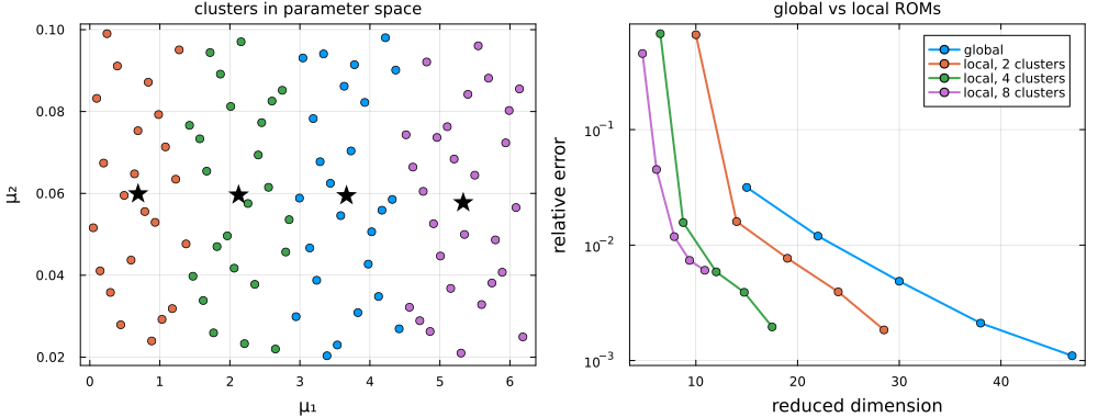
Here are the training parameters, coloured by cluster, together with the centroids:

using GridapROMs.ParamDataStructures: get_realisation, get_params

k, = get_clusters(local_rbop.trial.subspace)
μtrain = reduce(hcat,get_params(get_realisation(fesnaps)))
scatter(μtrain[1,:],μtrain[2,:];group=k.assignments,markersize=4,framestyle=:box,
  xlabel="μ₁",ylabel="μ₂",legend=:outerright,size=(600,350))
scatter!(k.centers[1,:],k.centers[2,:];marker=:star5,markersize=10,c=:black,label="centroids")

Since the parameter space is not rescaled, k-means splits it along $\mu_1$, which is the parameter that the solutions depend on the most.

Online, each parameter selects the cluster of its closest centroid, and the corresponding local reduced operator, a standard RBOperator, is extracted and solved:

using GridapROMs.RBSteady: get_local
μ1 = first(μon)
typeof(get_local(local_rbop,μ1))

GridapROMs.RBSteady.RBOperator{GridapROMs.ParamSteady.LinearParamEq, GridapROMs.Utils.Contribution{GridapROMs.RBSteady.GenericHRProjection{DEIMHyperReduction{GridapROMs.RBSteady.SearchSVDRank}, GridapROMs.RBSteady.ReducedAlgebraicProjection{Array{Float64, 3}}, GridapROMs.RBSteady.GreedyInterpolation{LinearAlgebra.LU{Float64, Matrix{Float64}, Vector{Int64}}, GridapROMs.RBSteady.GenericDomain{Gridap.Arrays.LazyArray{FillArrays.Fill{GridapROMs.RBSteady.CellsToIrowcolsMap{Gridap.Arrays.Table{Int32, Vector{Int32}, Vector{Int32}}, Gridap.Arrays.Table{Int32, Vector{Int32}, Vector{Int32}}, Vector{Int32}, Vector{Int64}, Vector{Int64}}, 1, Tuple{Base.OneTo{Int64}}}, Vector{Int32}, 1, Tuple{UnitRange{Int64}}}, Tuple{Vector{Int64}, Vector{Int64}}}}}, Gridap.Geometry.BodyFittedTriangulation{2, 2, Gridap.Geometry.CartesianDiscreteModel{2, Float64, typeof(identity)}, Gridap.Geometry.CartesianGrid{2, Float64, typeof(identity)}, Gridap.Arrays.IdentityVector{Int64}}}, GridapROMs.Utils.Contribution{GridapROMs.RBSteady.GenericHRProjection{DEIMHyperReduction{GridapROMs.RBSteady.SearchSVDRank}, GridapROMs.RBSteady.ReducedAlgebraicProjection{Matrix{Float64}}, GridapROMs.RBSteady.GreedyInterpolation{LinearAlgebra.LU{Float64, Matrix{Float64}, Vector{Int64}}, GridapROMs.RBSteady.GenericDomain{Gridap.Arrays.LazyArray{FillArrays.Fill{GridapROMs.RBSteady.CellsToIrowsMap{Gridap.Arrays.Table{Int32, Vector{Int32}, Vector{Int32}}, Vector{Int32}, Vector{Int64}}, 1, Tuple{Base.OneTo{Int64}}}, Vector{Int32}, 1, Tuple{UnitRange{Int64}}}, Vector{Int64}}}}, Gridap.Geometry.BodyFittedTriangulation{2, 2, Gridap.Geometry.CartesianDiscreteModel{2, Float64, typeof(identity)}, Gridap.Geometry.CartesianGrid{2, Float64, typeof(identity)}, Gridap.Arrays.IdentityVector{Int64}}}}

Local operators are saved and loaded exactly as global ones, with save and load_operator. They are compatible with all the features presented in Tutorial 2: TT-SVD, supremizer enrichment, linear/nonlinear splitting, transient problems, and the hyper-reduction strategies.

Accuracy versus dimension

Let us compare global and local ROMs for decreasing tolerances, as a function of the (average) dimension of the reduced subspaces:

tols = [3e-2,1e-2,3e-3,1e-3,3e-4]

function convergence(ncentroids)
  map(tols) do tol
    compression = ncentroids == 1 ? :global : :local
    red = Reduction(tol,H1();nparams=100,compression,ncentroids)
    rbs = RBSolver(solver,red;nparams_res=20,nparams_jac=60,verbose=false)
    op = reduced_operator(rbs,feop,fesnaps)
    x̂ = solution_snapshots(rbs,op,μon)
    projs = ncentroids == 1 ? [op.trial.subspace] : local_vals(op.trial.subspace)
    n = sum(p -> size(get_basis(p),2),projs) / length(projs)
    n,rom_performance(rbs,op,x,x̂).error
  end
end

plt = plot(;xlabel="reduced dimension",ylabel="relative error",yscale=:log10,
  framestyle=:box,size=(600,400))
for ncentroids in (1,2,4,8)
  res = convergence(ncentroids)
  label = ncentroids == 1 ? "global" : "local, $ncentroids clusters"
  plot!(plt,first.(res),last.(res);marker=:circle,lw=2,label)
end
plt

For a given dimension, local ROMs are considerably more accurate: equivalently, they reach a given accuracy with smaller (hence cheaper) reduced problems. The number of clusters is a trade-off: more clusters yield smaller local subspaces, but each of them is trained on fewer snapshots, which eventually limits the accuracy that can be reached. The function compute_ncentroids suggests a number of clusters from the training parameters, with an elbow criterion on the k-means variance:

compute_ncentroids(get_realisation(fesnaps))

10