Tutorial 2: Reduced order models
In this tutorial we learn
- what the offline and online phases of a ROM are, and why we separate them
- how to compress snapshots with POD and TT-SVD, in a norm of our choice
- how to hyper-reduce residuals and Jacobians with DEIM, S-OPT and RBF interpolation
- what a reduced operator is, and how to store it to file and load it back
- how to deal with multi-field (supremizer enrichment), nonlinear and transient problems
We assume you have gone through Tutorial 1.
Projection-based ROMs in a nutshell
Let $A_\mu u_\mu = b_\mu$ be the FE system of the parameterised problem, of size $N$. The solutions $\{u_\mu\}_{\mu \in \mathcal{D}}$ usually lie close to a low-dimensional subspace, spanned by the columns of a matrix $\Phi \in \mathbb{R}^{N \times n}$, with $n \ll N$. A reduced basis (RB) method seeks $u_\mu \approx \Phi \hat{u}_\mu$ by solving the $n \times n$ Galerkin system
\[\Phi^T A_\mu \Phi \, \hat{u}_\mu = \Phi^T b_\mu .\]
Solving this system is cheap, but assembling it is not: $A_\mu$ and $b_\mu$ still live in the FE space. Hyper-reduction removes this bottleneck, by approximating
\[A_\mu \approx \sum_{q=1}^{Q} \theta_q(\mu) A_q, \qquad b_\mu \approx \sum_{q=1}^{Q'} \vartheta_q(\mu) b_q,\]
where the coefficients $\theta, \vartheta$ are computed from a handful of entries of $A_\mu, b_\mu$. Only the cells supporting these entries (the reduced integration domain) are integrated online, and the projections $\Phi^T A_q \Phi$, $\Phi^T b_q$ are precomputed. The resulting workflow is split in two phases:
- offline (expensive, run once): compute FE snapshots, compress them into $\Phi$ (the reduction cycle), then compute residual and Jacobian snapshots and compress them into the affine expansions above (the hyper-reduction cycles). The output is a reduced operator.
- online (cheap, run for any new $\mu$): integrate on the reduced integration domains, assemble the $n \times n$ system, solve it.
Since the offline phase is the expensive one, the reduced operator can be saved to file, and loaded later in an online-only session.
The FE problem
We consider the Poisson problem of Tutorial 1:
using Gridap
using GridapROMs
using DrWatson
using Plots

pdomain = (1,10,1,10,1,10)
D = ParamSpace(pdomain)

κ(μ) = x -> 1 + μ[1]*exp(-x[1]*x[2])
κμ(μ) = parameterise(κ,μ)
g(μ) = x -> exp(-x[1]/μ[2])
gμ(μ) = parameterise(g,μ)
h(μ) = x -> 5*cos(μ[3]*x[1])
hμ(μ) = parameterise(h,μ)
f(x) = 10.0

model = CartesianDiscreteModel((0,1,0,1),(40,40))
Ω = Triangulation(model)
Γn = BoundaryTriangulation(model;tags=6)
dΩ = Measure(Ω,2)
dΓn = Measure(Γn,2)

reffe = ReferenceFE(lagrangian,Float64,1)
V = TestFESpace(Ω,reffe;conformity=:H1,dirichlet_tags=[1,2,3,5,7])
U = ParamTrialFESpace(V,gμ)

a(μ,u,v) = ∫(κμ(μ)*∇(v)⋅∇(u))dΩ
l(μ,v) = ∫(f*v)dΩ + ∫(hμ(μ)*v)dΓn
l (generic function with 1 method)There is one difference with respect to Tutorial 1: we tell the operator on which triangulations the right-hand side and the Jacobian are integrated, with a FEDomains structure:
domains = FEDomains((Ω,Γn),(Ω,))
feop = LinearParamOperator(l,a,D,U,V,domains)GenericParamOperator()This is the main API difference with respect to Gridap. GridapROMs hyper-reduces each integration domain separately: the residual is split into a volume contribution on Ω and a boundary contribution on Γn, and each of them gets its own affine expansion and its own reduced integration domain. Boundary terms are thus hyper-reduced with boundary cells only, and terms with a different parameter dependence are not mixed together, which keeps their expansions short.
The RB solver
An RBSolver collects the FE solver and the reduction strategies for the state, the residual and the Jacobian:
solver = LUSolver()

tol = 1e-4
state_reduction = Reduction(tol,H1();nparams=40)
rbsolver = RBSolver(solver,state_reduction;nparams_res=30,nparams_jac=20)RBSolver()State reduction
Reduction builds the strategy compressing the solution snapshots. Here, a truncated POD (PODReduction) retaining the modes needed to achieve a relative tolerance tol, computed from nparams=40 snapshots. Passing an integer instead of a float fixes the rank of the basis instead:
Reduction(10,H1();nparams=40)PODReduction{GridapROMs.RBSteady.FixedSVDRank, H1}(GridapROMs.RBSteady.FixedSVDRank(10), H1(), 40)The second argument is the norm in which the basis is orthonormal, and in which errors are measured. Available norms are
| Norm | Bilinear form |
|---|---|
EuclideanNorm | none: plain $\ell^2$ product of DOF vectors (default) |
L2 | $\int_\Omega u \cdot v$ |
H1 | $\int_\Omega u \cdot v + \nabla u : \nabla v$ |
EnergyNorm | any user-defined form (u,v) -> ∫(...)dΩ |
NitscheH1 | $H^1$ plus a Nitsche penalty on a boundary, for weakly imposed Dirichlet conditions |
BlockNorm | one of the above per field, in multi-field problems |
Working in a problem-specific norm (e.g. the energy norm of the PDE) yields reduced subspaces that are optimal in the norm that actually measures the error of the method.
Hyper-reduction
The keywords nparams_res and nparams_jac set how many residual and Jacobian snapshots are used in the hyper-reduction cycles. The hyper-reduction strategy is chosen with the keyword hypred_strategy:
hypred_strategy | Method | Online cost |
|---|---|---|
:deim (default) | DEIM, in its matrix version: greedy selection of interpolation entries | integration on the reduced domain |
:sopt | S-OPT: interpolation entries maximising the S-optimality criterion, more robust than the DEIM greedy | integration on the reduced domain |
:rbf | radial basis function interpolation of the coefficients $\theta(\mu)$: non-intrusive | no integration |
:none | no hyper-reduction: full assembly followed by a Galerkin projection | full integration |
:affine | the projections are computed once offline. Exact only for $\mu$-independent terms | no integration |
The tolerance of the hyper-reduction is the one of the state reduction. Different strategies (or tolerances) per term can be set by passing the reductions explicitly, e.g. to use :affine for a $\mu$-independent Jacobian:
using GridapROMs.RBSteady: HyperReduction
residual_reduction = HyperReduction(state_reduction;nparams=30)
jacobian_reduction = HyperReduction(state_reduction;hypred_strategy=:affine)
RBSolver(solver,state_reduction,residual_reduction,jacobian_reduction)
Offline phase
The offline phase is run with reduced_operator. We first compute the FE snapshots, so that we can reuse them later on:
fesnaps = solution_snapshots(rbsolver,feop)
rbop = reduced_operator(rbsolver,feop,fesnaps)RBOperator()Calling reduced_operator(rbsolver,feop) computes the snapshots internally. Under the hood, the function runs the reduction cycle and the hyper-reduction cycles:
Û,V̂ = reduced_spaces(rbsolver,feop,fesnaps)                 # state reduction
lhs,rhs = reduced_weak_form(rbsolver,feop,Û,V̂,fesnaps)      # hyper-reduction
rbop = ROMOperator(feop,Û,V̂,lhs,rhs)
The cost of each step is printed as it runs (pass verbose=false to the RBSolver to silence it). The singular values of the snapshots tell us how reducible the problem is:
using LinearAlgebra
σ = svdvals(collect(fesnaps))
plot(σ./σ[1];yscale=:log10,marker=:circle,legend=false,framestyle=:box,
  xlabel="index",ylabel="normalised singular value",size=(500,300))
The output is an RBOperator, with fields
op: the FE operatorfeoptrial,test: the reduced trial and test spaces, of typeRBSpacelhs,rhs: the hyper-reduced Jacobian and residual, with one entry per triangulation indomains
An RBOperator is itself a ParamOperator, which can be evaluated and solved exactly as its FE counterpart. The reduced spaces wrap the FE spaces together with the reduced basis $\Phi$:
Φ = get_basis(rbop.trial.subspace)
size(Φ)
(1600, 12)Saving and loading
The offline phase pays off when its output is reused across sessions. The reduced operator is saved with save, and loaded back with load_operator, given the FE operator:
dir = mktempdir()
save(dir,rbop)
readdir(dir)
4-element Vector{String}:
"contributions_lhs.jld"
"contributions_rhs.jld"
"projection_test.jld"
"projection_trial.jld"rbop = load_operator(dir,feop)RBOperator()A typical script loads the reduced operator if available, and runs the offline phase otherwise:
rbop = try
  load_operator(dir,feop)
catch
  rbop = reduced_operator(rbsolver,feop)
  save(dir,rbop)
  rbop
end
Snapshots can be saved and loaded in the same way, with save(dir,fesnaps) and load_snapshots.
Online phase
We now solve the reduced problem for new parameters. The first call compiles the online routines, so we time the second one:
μon = realisation(feop;nparams=10,sampling=:uniform)
x̂ = solution_snapshots(rbsolver,rbop,μon)
x̂ = solution_snapshots(rbsolver,rbop,μon)
1600×10 GridapROMs.ParamDataStructures.GenericSnapshots{Float64, 2, GridapROMs.DofMaps.VectorDofMap{1, Int64, LinearIndices{1, Tuple{Base.OneTo{Int64}}}}, Realisation{Vector{Vector{Float64}}}, Matrix{Float64}, GridapROMs.ParamDataStructures.ConsecutiveParamVector{Float64, Matrix{Float64}}}:
0.995552 1.00439 0.999211 0.988816 … 0.998806 0.998607 0.998879
0.990365 1.00724 0.99798 0.976291 0.997258 0.996795 0.997352
0.984821 1.00926 0.996523 0.963121 0.995525 0.994762 0.995616
0.979049 1.01073 0.994913 0.949621 0.993668 0.992582 0.99374
0.973119 1.01176 0.993189 0.935952 0.991719 0.990291 0.99176
0.967073 1.01247 0.991375 0.922213 … 0.989698 0.987912 0.989696
0.960938 1.01289 0.989488 0.908468 0.987618 0.985462 0.987566
0.954736 1.01307 0.987539 0.894762 0.985488 0.98295 0.985378
0.948481 1.01305 0.985538 0.881128 0.983315 0.980385 0.983142
0.942187 1.01284 0.983492 0.867591 0.981106 0.977774 0.980863
⋮ ⋱
1.09023 2.57763 1.64765 1.6794 0.980007 1.48319 0.99748
1.07292 2.52194 1.6702 1.74416 0.975508 1.47831 0.989857
1.05731 2.45997 1.68789 1.8088 0.972204 1.47309 0.983445
1.0436 2.3959 1.70058 1.87146 0.970069 1.4677 0.978294
1.032 2.33402 1.70835 1.93007 … 0.969032 1.46231 0.974418
1.0227 2.27858 1.71161 1.98233 0.968957 1.45718 0.971789
1.01584 2.23361 1.71113 2.02557 0.969628 1.45259 0.970318
1.01159 2.20296 1.70822 2.05653 0.970698 1.44901 0.969828
1.01011 2.19111 1.70581 2.06948 0.971422 1.44735 0.969887To assess the quality of the ROM we compute the FE solutions too, and compare them with rom_performance, which returns the relative error (in the norm of the reduction) and the speedup of the online phase with respect to the FE solver:
x = solution_snapshots(rbsolver,feop,μon)
rom_performance(rbsolver,rbop,x,x̂)
----------------------- ROM results -------------------------
> error: 0.00034486470351887956
> speedup in time: 10.84650756560604
> speedup in memory: 7.936578042421967
-------------------------------------------------------------
On this small problem the speedup is modest: it grows with the size of the FE problem (see the Navier-Stokes example below). Reduced solutions are FE functions like any other:
using GridapROMs.ParamDataStructures: get_param_data
uh = FEFunction(U(μon),get_param_data(x))
ûh = FEFunction(U(μon),get_param_data(x̂))

function plot_field(uh;n=101,kwargs...)
  xs = range(0,1;length=n)
  pts = [Point(x,y) for x in xs, y in xs]
  vals = reshape(uh(vec(pts)),n,n)
  heatmap(xs,xs,permutedims(vals);aspect_ratio=:equal,framestyle=:box,
    xlims=(0,1),ylims=(0,1),c=:viridis,titlefontsize=10,kwargs...)
end

uh1 = param_getindex(uh,1)
ûh1 = param_getindex(ûh,1)
plot(
  plot_field(uh1;title="FE"),
  plot_field(ûh1;title="ROM"),
  plot_field(abs∘(uh1-ûh1);title="|FE - ROM|",c=:inferno);
  layout=(1,3),size=(1100,300),right_margin=5Plots.mm)
Accuracy of the hyper-reduction strategies
We compare the hyper-reduction strategies for decreasing tolerances. All the ROMs are trained on the same snapshots, which we pass to reduced_operator:
tols = [1e-1,1e-2,1e-3,1e-4,1e-5]
strategies = (:deim,:sopt,:rbf,:none)

errors = map(strategies) do strategy
  map(tols) do tol
    red = Reduction(tol,H1();nparams=40)
    rbs = RBSolver(solver,red;nparams_res=30,nparams_jac=20,hypred_strategy=strategy,verbose=false)
    op = reduced_operator(rbs,feop,fesnaps)
    x̂ = solution_snapshots(rbs,op,μon)
    rom_performance(rbs,op,x,x̂).error
  end
end

plt = plot(tols,tols;lw=2,ls=:dash,c=:black,label="tolerance",xscale=:log10,yscale=:log10,
  xflip=true,xlabel="tolerance",ylabel="relative error",framestyle=:box,legend=:topright,
  size=(600,400))
for (strategy,err) in zip(strategies,errors)
  plot!(plt,tols,err;marker=:circle,lw=2,label=string(strategy))
end
plt
DEIM and S-OPT (indistinguishable here) follow the prescribed tolerance. Without hyper-reduction the error is smallest, at the price of a full assembly online. RBF interpolation saturates, since the coefficients $\theta(\mu)$ are interpolated from 30 samples only; in exchange, its online phase requires no integration at all.
Tensor-train reduction
On Cartesian geometries, snapshots can be reshaped as tensors, with one dimension per spatial direction and one for the parameter. The TT-SVD compresses each dimension sequentially, producing a basis in tensor-train format, which is much cheaper to compute and store than a POD basis on fine meshes. Hyper-reduction is performed with the TT-DEIM.
All we need is a TProductDiscreteModel, which stores the 1D models whose tensor product is the 2D model, and a vector of tolerances, one per dimension of the snapshots:
model_tt = TProductDiscreteModel((0,1,0,1),(40,40))
Ω_tt = Triangulation(model_tt)
Γn_tt = BoundaryTriangulation(model_tt;tags=6)
dΩ_tt = Measure(Ω_tt,2)
dΓn_tt = Measure(Γn_tt,2)

V_tt = TestFESpace(Ω_tt,reffe;conformity=:H1,dirichlet_tags=[1,2,3,5,7])
U_tt = ParamTrialFESpace(V_tt,gμ)

a_tt(μ,u,v) = ∫(κμ(μ)*∇(v)⋅∇(u))dΩ_tt
l_tt(μ,v) = ∫(f*v)dΩ_tt + ∫(hμ(μ)*v)dΓn_tt
feop_tt = LinearParamOperator(l_tt,a_tt,D,U_tt,V_tt,FEDomains((Ω_tt,Γn_tt),(Ω_tt,)))

state_reduction_tt = Reduction(fill(tol,3),H1();nparams=40)
TTSVDReduction{H1}(GridapROMs.RBSteady.TTSVDRanks(GridapROMs.RBSteady.SearchSVDRank[GridapROMs.RBSteady.SearchSVDRank(6.933612743506348e-5), GridapROMs.RBSteady.SearchSVDRank(6.933612743506348e-5), GridapROMs.RBSteady.SearchSVDRank(6.933612743506348e-5)]), H1(), 40)A vector of tolerances gives a TTSVDReduction. The rest is unchanged:
rbsolver_tt = RBSolver(solver,state_reduction_tt;nparams_res=30,nparams_jac=20,verbose=false)
fesnaps_tt = solution_snapshots(rbsolver_tt,feop_tt)
size(fesnaps_tt)
(40, 40, 40)The snapshots are now a 40 × 40 × 40 tensor: free DOFs in $x$, in $y$, and parameters.
rbop_tt = reduced_operator(rbsolver_tt,feop_tt,fesnaps_tt)
size.(get_cores(rbop_tt.trial.subspace))
2-element Vector{Tuple{Int64, Int64, Int64}}:
(1, 40, 10)
(10, 40, 13)x_tt = solution_snapshots(rbsolver_tt,feop_tt,μon)
x̂_tt = solution_snapshots(rbsolver_tt,rbop_tt,μon)
rom_performance(rbsolver_tt,rbop_tt,x_tt,x̂_tt) ----------------------- ROM results -------------------------
> error: 0.0003139615777934504
> speedup in time: 0.02917640521735174
> speedup in memory: 0.2808762607965919
-------------------------------------------------------------
Multi-field and nonlinear problems
We now reduce a steady Navier-Stokes problem: the lid-driven cavity, with parameterised viscosity $\nu = \mu_1/100$ and lid velocity $u_{lid}(x) = 16\mu_2 x_1^2(1-x_1)^2$. Velocity and pressure are discretised with Taylor-Hood elements, and the pressure is fixed at the bottom-left corner:
using GridapSolvers
using GridapSolvers.NonlinearSolvers
using Gridap.MultiField: BlockMultiFieldStyle

D_ns = ParamSpace((1.0,10.0,0.5,1.5))

model_ns = CartesianDiscreteModel((0,1,0,1),(20,20))
Ω_ns = Triangulation(model_ns)
dΩ_ns = Measure(Ω_ns,4)

ν(μ) = x -> μ[1]/100*exp(-x[1])
νμ(μ) = parameterise(ν,μ)
g_ns(μ) = x -> VectorValue(16*μ[2]*x[1]^2*(1-x[1])^2,0.0)*(x[2]==1.0)
g_nsμ(μ) = parameterise(g_ns,μ)

reffe_u = ReferenceFE(lagrangian,VectorValue{2,Float64},2)
reffe_p = ReferenceFE(lagrangian,Float64,1)
V_u = TestFESpace(Ω_ns,reffe_u;conformity=:H1,dirichlet_tags=[1,2,3,4,5,6,7,8])
V_p = TestFESpace(Ω_ns,reffe_p;conformity=:H1,dirichlet_tags=[1])
U_u = ParamTrialFESpace(V_u,g_nsμ)
U_p = ParamTrialFESpace(V_p)
Y = MultiFieldFESpace([V_u,V_p];style=BlockMultiFieldStyle())
X = MultiFieldFESpace([U_u,U_p];style=BlockMultiFieldStyle())MultiFieldFESpace()Linear/nonlinear splitting
The Stokes terms are linear in the unknowns, while the convective term is not. Assembling the linear terms at every Newton iteration is a waste, in the FE and even more so in the ROM. In GridapROMs we write the two parts separately, and gather them in a Bundle:
- the linear part is written as in a
LinearParamOperator: a right-hand siderhs(μ,v)and a bilinear formjac(μ,du,v) - the nonlinear part is written as in a
ParamOperator: a residualres(μ,u,v)and its Jacobianjac(μ,u,du,v)
conv(u,∇u) = (∇u')⋅u
dconv(du,∇du,u,∇u) = conv(u,∇du)+conv(du,∇u)

rhs_lin(μ,(v,q)) = ∫(VectorValue(0.0,0.0)⋅v)dΩ_ns
jac_lin(μ,(du,dp),(v,q)) = ∫(νμ(μ)*∇(v)⊙∇(du))dΩ_ns - ∫(dp*(∇⋅(v)))dΩ_ns + ∫(q*(∇⋅(du)))dΩ_ns

res_nlin(μ,(u,p),(v,q)) = ∫(v⊙(conv∘(u,∇(u))))dΩ_ns
jac_nlin(μ,(u,p),(du,dp),(v,q)) = ∫(v⊙(dconv∘(du,∇(du),u,∇(u))))dΩ_ns

res = Bundle(rhs_lin,res_nlin)
jac = Bundle(jac_lin,jac_nlin)
domains_ns = Bundle(FEDomains((Ω_ns,),(Ω_ns,)),FEDomains((Ω_ns,),(Ω_ns,)))
feop_ns = ParamOperator(res,jac,D_ns,X,Y,domains_ns)GenericParamOperator()The linear and nonlinear parts are hyper-reduced independently. Online, the linear part is assembled once per parameter, and only the nonlinear part is updated at each Newton iteration.
Supremizer enrichment
A Galerkin projection of a saddle-point problem is not inf-sup stable in general: the reduced velocity space may be too poor to control the reduced pressures. The supremizer enrichment fixes this, by adding to the velocity basis the supremizers of the pressure basis, i.e. the solutions of $X_u s_i = B^T \phi^p_i$, where $X_u$ is the velocity norm matrix and $B^T$ the pressure-velocity coupling. A SupremizerReduction wraps any reduction, given the coupling operator, here DivCoupling ($\int_\Omega p \, \nabla \cdot v$):
state_reduction_ns = SupremizerReduction(DivCoupling(),1e-4,BlockNorm((H1(),L2()));nparams=30)

fesolver_ns = NewtonSolver(LUSolver();rtol=1e-10,maxiter=20,verbose=false)
rbsolver_ns = RBSolver(fesolver_ns,state_reduction_ns;nparams_res=20,nparams_jac=20,verbose=false)

fesnaps_ns = solution_snapshots(rbsolver_ns,feop_ns)
rbop_ns = reduced_operator(rbsolver_ns,feop_ns,fesnaps_ns)

μon_ns = realisation(feop_ns;nparams=5,sampling=:uniform)
x̂_ns = solution_snapshots(rbsolver_ns,rbop_ns,μon_ns)
x_ns = solution_snapshots(rbsolver_ns,feop_ns,μon_ns)
x̂_ns = solution_snapshots(rbsolver_ns,rbop_ns,μon_ns)
rom_performance(rbsolver_ns,rbop_ns,x_ns,x̂_ns)
----------------------- ROM results -------------------------
> error: [0.000198139615982057, 0.00016028952588392124]
> speedup in time: 265.0682018854342
> speedup in memory: 49.80678848047198
-------------------------------------------------------------
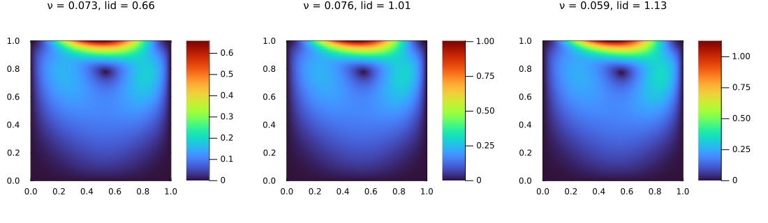
The error is reported per field (velocity, pressure). Let us look at the reduced velocity for three of the online parameters:
ûh_ns = FEFunction(U_u(μon_ns),get_param_data(x̂_ns[1]))
plts = map(Iterators.take(enumerate(μon_ns),3)) do (i,μi)
  plot_field(norm∘param_getindex(ûh_ns,i);c=:turbo,
    title="ν = $(round(μi[1]/100;digits=3)), lid = $(round(μi[2];digits=2))")
end
plot(plts...;layout=(1,3),size=(1100,320))
Transient problems
Transient problems are reduced in space and time. For the heat equation of Tutorial 1 (with the domains, this time):
gt(μ,t) = x -> exp(-x[1]/μ[2])*sin(π*t)
gμt(μ,t) = parameterise(gt,μ,t)
ht(μ,t) = x -> 5*cos(μ[3]*x[1])*sin(π*t)
hμt(μ,t) = parameterise(ht,μ,t)
κt(μ,t) = x -> 1 + μ[1]*exp(-x[1]*x[2])
κμt(μ,t) = parameterise(κt,μ,t)

dt = 0.05
t0,tf = 0.0,1.0
Dt = TransientParamSpace(pdomain,t0:dt:tf)
Ut = TransientTrialParamFESpace(V,gμt)

stiffness(μ,t,u,v) = ∫(κμt(μ,t)*∇(v)⋅∇(u))dΩ
mass(μ,t,uₜ,v) = ∫(v*uₜ)dΩ
rhs(μ,t,v) = ∫(f*v)dΩ + ∫(hμt(μ,t)*v)dΓn

domains_t = FEDomains((Ω,Γn),((Ω,),(Ω,)))
feop_t = TransientLinearParamOperator(rhs,(stiffness,mass),Dt,Ut,V,domains_t)

fesolver_t = ThetaMethod(LUSolver(),dt,0.5)
u0(μ) = x -> 0.0
u0μ(μ) = parameterise(u0,μ)
uh0μ(μ) = interpolate_everywhere(u0μ(μ),Ut(μ,t0))
uh0μ (generic function with 1 method)Note that the Jacobian domains are a tuple, one entry per Jacobian (stiffness and mass). A TransientReduction compresses the snapshots in space and in time:
- with a tolerance (or rank), a space-time POD, i.e. a Kronecker product of a spatial and a temporal basis
- with a vector of tolerances, a TT-SVD (requires a
TProductDiscreteModel)
The number of Jacobian snapshots is given per Jacobian, with nparams_jacs. The mass matrix does not depend on the parameter, so one snapshot suffices:
state_reduction_t = TransientReduction(1e-4,H1();nparams=20)
rbsolver_t = RBSolver(fesolver_t,state_reduction_t;nparams_res=15,nparams_jacs=(15,1),verbose=false)

fesnaps_t = solution_snapshots(rbsolver_t,feop_t,uh0μ)
rbop_t = reduced_operator(rbsolver_t,feop_t,fesnaps_t)

μon_t = realisation(feop_t;nparams=5,sampling=:uniform)
x̂_t = solution_snapshots(rbsolver_t,rbop_t,μon_t,uh0μ)
x_t = solution_snapshots(rbsolver_t,feop_t,μon_t,uh0μ)
x̂_t = solution_snapshots(rbsolver_t,rbop_t,μon_t,uh0μ)
rom_performance(rbsolver_t,rbop_t,x_t,x̂_t)
----------------------- ROM results -------------------------
> error: 0.00029395324149232533
> speedup in time: 2.6594823720398124
> speedup in memory: 6.965897622233239
-------------------------------------------------------------
Since the reduced basis spans space and time, the online phase solves a single space-time system, without time marching.
Summary
| Step | Function |
|---|---|
| define the FE problem, with its integration domains | FEDomains, LinearParamOperator, ParamOperator, Bundle |
| choose the reductions | Reduction, SupremizerReduction, TransientReduction, RBSolver |
| offline phase | solution_snapshots, reduced_operator |
| store and retrieve | save, load_operator, load_snapshots |
| online phase | solution_snapshots, rom_performance |
In the next tutorial we improve the accuracy of the ROM with local reduced operators.