Tutorial 14: On using DrWatson.jl

In this tutorial, we will learn

How to use DrWatson.jl to accelerate and reproduce our Gridap simulation workflows

DrWatson.jl is a Julia package that helps managing a typical scientific workflow thorought all its phases, see a summary here.

All its functionalities can be accessed with (non-invasive) simple function calls.

In order to illustrate how to benefit from DrWatson.jl in Gridap.jl simulations, we refactor here the convergence test from the Code validation tutorial.

Instead of implementing a helper function to carry out the convergence test, we will generate them using DrWatson.jl functions.

1. Activate your project

The first step is to activate our project using quickactivate. This does not only activate the project, it also sets the relative paths within the project, so you can safely use the functions projectdir() and its derivatives datadir(), plotsdir(), srcdir(), etc. Beware of this warning, you must activate the project before using other packages.

using DrWatson
@quickactivate "Tutorials"

Although this tutorial is already in a Project (and git repo), we could also start our scientific project from scratch with DrWatson.jl, using function initialize_project. This function initiates, on the working directory, (1) a git repo with a folder structure enriched for scientific workflows, e.g. folders data, plots, papers, etc., and (2)Project.toml and Manifest.toml files. More details here.

Once the project is activated, we ensure that all packages we use have the versions dictated by our activated project.

using Gridap
import Gridap: ∇

2. Prepare the simulations

We consider the Poisson equation in the unit square $\Omega\doteq (0,1)^2$ as a model problem,

\[\left\lbrace \begin{aligned} -\Delta u = f \ \text{in} \ \Omega\\ u = g \ \text{on}\ \partial\Omega.\\ \end{aligned} \right.\]

We are going to perform a convergence test with the manufactured solution $u(x) = x_1^3 + x_2^3$.

To this end, we want to solve our computational model for many combinations of mesh size and order of FE approximation (parameters) and extract the L2- and H1-norm errors (output data).

We first group all parameters and parameter values in a single ditionary

params = Dict(
  "cells_per_axis" => [8,16,32,64],
  "fe_order" => [1,2]
)

and then we use DrWatson's dict_list to expand all the parameters into a vector of dictionaries. Each dictionary contains the parameter-value combinations corresponding to a single simulation case.

dicts = dict_list(params)

Warning! Be careful when combining parameters of different value type. You may end up with dictionaries that do not have a concrete type and experience a significant type-inference overhead when running the simulations.

We wrap next in a function a run of our computational model for a single pair (cells_per_axis,fe_order). The function returns the L2- and H1-error norms.

We define the manufactured function, as usual

p = 3
u(x) = x[1]^p+x[2]^p
∇u(x) = VectorValue(p*x[1]^(p-1),p*x[2]^(p-1))
f(x) = -p*(p-1)*(x[1]^(p-2)+x[2]^(p-2))
∇(::typeof(u)) = ∇u

And the function that runs a single case of our parametric space reads

function run(n::Int,k::Int)

  domain = (0,1,0,1)
  partition = (n,n)
  model = CartesianDiscreteModel(domain,partition)

  reffe = ReferenceFE(lagrangian,Float64,k)
  V0 = TestFESpace(model,reffe,conformity=:H1,dirichlet_tags="boundary")
  U = TrialFESpace(V0,u)

  degree = 2*p
  Ω = Triangulation(model)
  dΩ = Measure(Ω,degree)

  a(u,v) = ∫( ∇(u)⊙∇(v) ) * dΩ
  b(v) = ∫( v*f ) * dΩ

  op = AffineFEOperator(a,b,U,V0)

  uh = solve(op)

  e = u - uh

  el2 = sqrt(sum( ∫( e*e )*dΩ ))
  eh1 = sqrt(sum( ∫( e*e + ∇(e)⋅∇(e) )*dΩ ))

  (el2, eh1)

end

In order to communicate with DrWatson.jl helper functions, we need to add an extra layer on top of run, such that the input and output are dictionaries.

Note the use of functions @unpack and @dict to decompose and compose the dictionaries. You can check in DrWatson.jl's documentation further functions to manipulate dictionaries.

function run(case::Dict)
  @unpack cells_per_axis, fe_order = case
  el2, eh1 = run(cells_per_axis,fe_order)
  h = 1.0/cells_per_axis
  results = @strdict el2 eh1 h
  merge(case,results)
end

3. Run and save

While running the simulations, we need to save the results. DrWatson.jl frees you from the burden of generating the filenames for each case. For this purpose, it provides the functions savename, @tagsave or produceorload, among others.

Among them, we recommend using produceorload. The special feature of this function is that it checks whether the file containing the output data of the case already exists. If that happens, then the function loads the file, instead of running the case. In this way, we avoid repeating simulations that have already been run.

Thus, in order to run all simulation cases, it suffices to map all cases in dicts to the produce_or_load function:

function run_or_load(case::Dict)
  produce_or_load(
    projectdir("assets","validation_DrWatson"),
    case,
    run,
    prefix="res",
    tag=true,
    verbose=true
  )
  return true
end

map(run_or_load,dicts)

Note that the results of each case are stored in a binary database file in the projectdir("assets","validation_DrWatson") folder. Each result file stores the output dictionary that returns from run(case).

We also observe that we set tag=true in produce_or_load. This option is key to preserve reproducibility. It adds to the output dictionary the field :gitcommit, thus allowing us to trace the status of the code, at which we obtained those results. Furthermore, if the git repo is dirty, one more field :gitpatch is added, storing the difference string.

In some situations, you will prefer to repeat all simulations and track their evolution as you change the code. To this end, check out safesave.

4. Listing the simulations

Results stored by DrWatson.jl in databases are handled with the DataFrames.jl package, a powerful Julia package to manipulate tabular data.

using DataFrames

To collect all simulation results, it suffices to use the collect_results! function from DrWatson.jl from the folder where the results are stored.

df = collect_results(projectdir("assets","validation_DrWatson"))

We order next the database by (ascending) mesh size and we extract the arrays of mesh sizes and errors

sort!(df,:h)
hs = df[(df.fe_order .== 1),:h]
el2s1 = df[(df.fe_order .== 1),:el2]
eh1s1 = df[(df.fe_order .== 1),:eh1]
el2s2 = df[(df.fe_order .== 2),:el2]
eh1s2 = df[(df.fe_order .== 2),:eh1]

5. Generate the plot

With the generated data, we do the classical convergence plot and interpret it in the same way as in the validation tutorial.

using Plots

plot(hs,[el2s1 eh1s1 el2s2 eh1s2],
    xaxis=:log, yaxis=:log,
    label=["L2 k=1" "H1 k=1" "L2 k=2" "H1 k=2"],
    shape=:auto,
    xlabel="h",ylabel="error norm")

If you run the code in a notebook, you will see a figure like this one: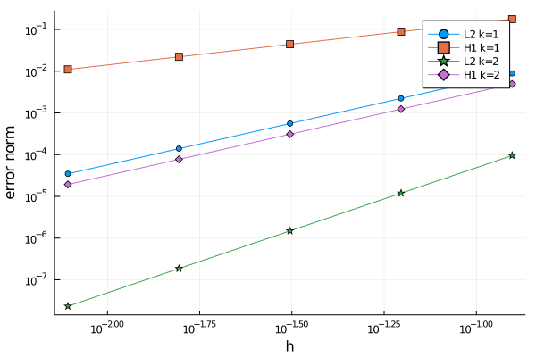

Congrats, another tutorial done!

If you use DrWatson.jl in a scientific project that leads to a publication, please do not forget to cite the paper associated with it:

@article{Datseris2020,
 doi = {10.21105/joss.02673},
 url = {https://doi.org/10.21105/joss.02673},
 year = {2020},
 publisher = {The Open Journal},
 volume = {5},
 number = {54},
 pages = {2673},
 author = {George Datseris and Jonas Isensee and Sebastian Pech and Tamás Gál},
 title = {DrWatson: the perfect sidekick for your scientific inquiries},
 journal = {Journal of Open Source Software}
}

This page was generated using Literate.jl.