Tutorial 8: Incompressible Navier-Stokes
![]()
![]()
In this tutorial, we will learn
- How to solve nonlinear multi-field PDEs in Gridap
- How to build FE spaces whose functions have zero mean value
Problem statement
The goal of this last tutorial is to solve a nonlinear multi-field PDE. As a model problem, we consider a well known benchmark in computational fluid dynamics, the lid-driven cavity for the incompressible Navier-Stokes equations. Formally, the PDE we want to solve is: find the velocity vector $u$ and the pressure $p$ such that
\[\left\lbrace \begin{aligned} -\Delta u + \mathit{Re}\ (u\cdot \nabla)\ u + \nabla p = 0 &\text{ in }\Omega,\\ \nabla\cdot u = 0 &\text{ in } \Omega,\\ u = g &\text{ on } \partial\Omega, \end{aligned} \right.\]
where the computational domain is the unit square $\Omega \doteq (0,1)^d$, $d=2$, $\mathit{Re}$ is the Reynolds number (here, we take $\mathit{Re}=10$), and $(w \cdot \nabla)\ u = (\nabla u)^t w$ is the well known convection operator. In this example, the driving force is the Dirichlet boundary velocity $g$, which is a non-zero horizontal velocity with a value of $g = (1,0)^t$ on the top side of the cavity, namely the boundary $(0,1)\times\{1\}$, and $g=0$ elsewhere on $\partial\Omega$. Since we impose Dirichlet boundary conditions on the entire boundary $\partial\Omega$, the mean value of the pressure is constrained to zero in order have a well posed problem,
\[\int_\Omega q \ {\rm d}\Omega = 0.\]
Numerical Scheme
In order to approximate this problem we chose a formulation based on inf-sub stable $Q_k/P_{k-1}$ elements with continuous velocities and discontinuous pressures (see, e.g., [1] for specific details). The interpolation spaces are defined as follows. The velocity interpolation space is
\[V \doteq \{ v \in [C^0(\Omega)]^d:\ v|_T\in [Q_k(T)]^d \text{ for all } T\in\mathcal{T} \},\]
where $T$ denotes an arbitrary cell of the FE mesh $\mathcal{T}$, and $Q_k(T)$ is the local polynomial space in cell $T$ defined as the multi-variate polynomials in $T$ of order less or equal to $k$ in each spatial coordinate. Note that, this is the usual continuous vector-valued Lagrangian FE space of order $k$ defined on a mesh of quadrilaterals or hexahedra. On the other hand, the space for the pressure is
\[\begin{aligned} Q_0 &\doteq \{ q \in Q: \ \int_\Omega q \ {\rm d}\Omega = 0\}, \text{ with}\\ Q &\doteq \{ q \in L^2(\Omega):\ q|_T\in P_{k-1}(T) \text{ for all } T\in\mathcal{T}\}, \end{aligned}\]
where $P_{k-1}(T)$ is the polynomial space of multi-variate polynomials in $T$ of degree less or equal to $k-1$. Note that functions in $Q_0$ are strongly constrained to have zero mean value. This is achieved in the code by removing one degree of freedom from the (unconstrained) interpolation space $Q$ and adding a constant to the computed pressure so that the resulting function has zero mean value.
The weak form associated to these interpolation spaces reads: find $(u,p)\in U_g \times Q_0$ such that $[r(u,p)](v,q)=0$ for all $(v,q)\in V_0 \times Q_0$ where $U_g$ and $V_0$ are the set of functions in $V$ fulfilling the Dirichlet boundary condition $g$ and $0$ on $\partial\Omega$ respectively. The weak residual $r$ evaluated at a given pair $(u,p)$ is the linear form defined as
\[[r(u,p)](v,q) \doteq a((u,p),(v,q))+ [c(u)](v),\]
with
\[\begin{aligned} a((u,p),(v,q)) &\doteq \int_{\Omega} \nabla v \cdot \nabla u \ {\rm d}\Omega - \int_{\Omega} (\nabla\cdot v) \ p \ {\rm d}\Omega + \int_{\Omega} q \ (\nabla \cdot u) \ {\rm d}\Omega,\\ [c(u)](v) &\doteq \int_{\Omega} v \cdot \left( (u\cdot\nabla)\ u \right)\ {\rm d}\Omega.\\ \end{aligned}\]
Note that the bilinear form $a$ is associated with the linear part of the PDE, whereas $c$ is the contribution to the residual resulting from the convective term.
In order to solve this nonlinear weak equation with a Newton-Raphson method, one needs to compute the Jacobian associated with the residual $r$. In this case, the Jacobian $j$ evaluated at a pair $(u,p)$ is the bilinear form defined as
\[[j(u,p)]((\delta u, \delta p),(v,q)) \doteq a((\delta u,\delta p),(v,q)) + [{\rm d}c(u)](\delta u,v),\]
where ${\rm d}c$ results from the linearization of the convective term, namely
\[[{\rm d}c(u)](\delta u,v) \doteq \int_{\Omega} v \cdot \left( (u\cdot\nabla)\ \delta u \right) \ {\rm d}\Omega + \int_{\Omega} v \cdot \left( (\delta u\cdot\nabla)\ u \right) \ {\rm d}\Omega.\]
The implementation of this numerical scheme is done in Gridap by combining the concepts previously seen for single-field nonlinear PDEs and linear multi-field problems.
Discrete model
We start with the discretization of the computational domain. We consider a $100\times100$ Cartesian mesh of the unit square.
using Gridap
n = 100
domain = (0,1,0,1)
partition = (n,n)
model = CartesianDiscreteModel(domain,partition)
For convenience, we create two new boundary tags, namely "diri1" and "diri0", one for the top side of the square (where the velocity is non-zero), and another for the rest of the boundary (where the velocity is zero).
labels = get_face_labeling(model)
add_tag_from_tags!(labels,"diri1",[6,])
add_tag_from_tags!(labels,"diri0",[1,2,3,4,5,7,8])
FE spaces
For the velocities, we need to create a conventional vector-valued continuous Lagrangian FE space. In this example, we select a second order interpolation.
D = 2
order = 2
reffeᵤ = ReferenceFE(lagrangian,VectorValue{2,Float64},order)
V = TestFESpace(model,reffeᵤ,conformity=:H1,labels=labels,dirichlet_tags=["diri0","diri1"])
The interpolation space for the pressure is built as follows
reffeₚ = ReferenceFE(lagrangian,Float64,order-1;space=:P)
Q = TestFESpace(model,reffeₚ,conformity=:L2,constraint=:zeromean)
With the options :Lagrangian, space=:P, valuetype=Float64, and order=order-1, we select the local polynomial space $P_{k-1}(T)$ on the cells $T\in\mathcal{T}$. With the symbol space=:P we specifically chose a local Lagrangian interpolation of type "P". Without using space=:P, would lead to a local Lagrangian of type "Q" since this is the default for quadrilateral or hexahedral elements. On the other hand, constraint=:zeromean leads to a FE space, whose functions are constrained to have mean value equal to zero, which is just what we need for the pressure space. With these objects, we build the trial multi-field FE spaces
uD0 = VectorValue(0,0)
uD1 = VectorValue(1,0)
U = TrialFESpace(V,[uD0,uD1])
P = TrialFESpace(Q)

Y = MultiFieldFESpace([V, Q])
X = MultiFieldFESpace([U, P])
scale_dof is not used here, because currently $H^1$ and $L^2$ conforming elements both use the same Piola map in Gridap (the trivial one).
Triangulation and integration quadrature
From the discrete model we can define the triangulation and integration measure
degree = order
Ωₕ = Triangulation(model)
dΩ = Measure(Ωₕ,degree)
Nonlinear weak form
The different terms of the nonlinear weak form for this example are defined following an approach similar to the one discussed for the $p$-Laplacian equation, but this time using the notation for multi-field problems.
const Re = 10.0
conv(u,∇u) = Re*(∇u')⋅u
dconv(du,∇du,u,∇u) = conv(u,∇du)+conv(du,∇u)
The bilinear form reads
a((u,p),(v,q)) = ∫( ∇(v)⊙∇(u) - (∇⋅v)*p + q*(∇⋅u) )dΩThe nonlinear term and its Jacobian are given by
c(u,v) = ∫( v⊙(conv∘(u,∇(u))) )dΩ
dc(u,du,v) = ∫( v⊙(dconv∘(du,∇(du),u,∇(u))) )dΩ
Finally, the Navier-Stokes weak form residual and Jacobian can be defined as
res((u,p),(v,q)) = a((u,p),(v,q)) + c(u,v)
jac((u,p),(du,dp),(v,q)) = a((du,dp),(v,q)) + dc(u,du,v)
With the functions res, and jac representing the weak residual and the Jacobian, we build the nonlinear FE problem:
op = FEOperator(res,jac,X,Y)Nonlinear solver phase
To finally solve the problem, we consider the same nonlinear solver as previously considered for the $p$-Laplacian equation.
using LineSearches: BackTracking
nls = NLSolver(
  show_trace=true, method=:newton, linesearch=BackTracking())
solver = FESolver(nls)
In this example, we solve the problem without providing an initial guess (a default one equal to zero will be generated internally)
uh, ph = solve(solver,op)Finally, we write the results for visualization (see next figure).
mkpath("output_path")
writevtk(Ωₕ,"output_path/ins-results",cellfields=["uh"=>uh,"ph"=>ph])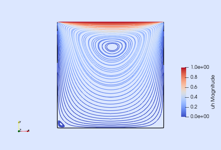
References
[1] H. C. Elman, D. J. Silvester, and A. J. Wathen. Finite elements and fast iterative solvers: with applications in incompressible fluid dynamics. Oxford University Press, 2005.
This page was generated using Literate.jl.