28-29th, November, 2023 | Australian National University, Canberra
In this tutorial, we will use the MPI-emulated environment provided by DebugArray to interactively have a look at some key aspects of how GridapDistributed works.
We will be using three packages:
Gridap, which provides the local FE framework
PartitionedArrays, which provides a generic library for MPI-distributed linear algebra
GridapDistributed, which provides the distributed layer on top of Gridap
using Gridap
using GridapDistributed
using PartitionedArrays
We start by creating our distributed rank indices, which plays the role of the more traditional communicator (such as MPI.COMM_WORLD).
nprocs = (2,1)
ranks  = with_debug() do distribute
  distribute(LinearIndices((prod(nprocs),)))
endWe can create a distributed Cartesian model by passing the newly-created ranks to the serial constructor. Thanks to Julia's multiple-dispatch, this is pretty much the only change we will have to do to convert a serial Gridap code into a GridapDistributed code.
domain = (0,1,0,1)
ncells = (4,2)
serial_model = CartesianDiscreteModel(domain,ncells)

model = CartesianDiscreteModel(ranks,nprocs,domain,ncells)
The created DistributedDiscreteModel is just a wrapper around a distributed array of serial models. One can get access to the local models with the method local_views, which is defined for most distributed structures in GridapDistributed.
local_models = local_views(model)
display(local_models)
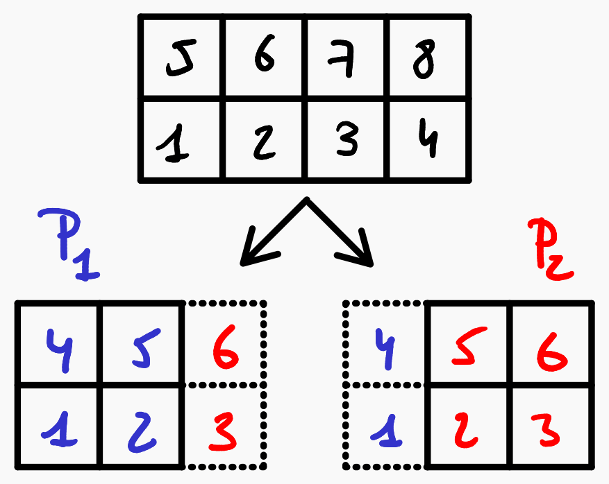
A key aspect in parallel programming is the concept of owned & ghost ids. If we compare the number of cells of the distributed model to the number of cells of the local model portions, we can observe that the local models overlap:
global_ncells = num_cells(model)
local_ncells  = map(num_cells,local_views(model))
This overlap is due to ghost cells. The Owned/Ghost layout of the current distributed model can be seen in the next figure:

This information is also stored on the distributed model, and can be accessed in the following way:
cell_gids = get_cell_gids(model)
local_cell_to_global_cell = map(local_to_global,partition(cell_gids))
local_cell_to_owner       = map(local_to_owner,partition(cell_gids))
owned_cell_to_local_cell  = map(own_to_local,partition(cell_gids))
ghost_cell_to_local_cell  = map(ghost_to_local,partition(cell_gids))
For each processor, we have
local_to_global - map from local cell ids to global cell ids
local_to_owner - map from local cell ids to the processor id of the cell owner
own_to_local - list of owned local cells
ghost_to_local - list of ghost local cells
More documentation on this can be found in PartitionedArrays.jl
We can then continue by creating a DistributedFESpace, which (like DistributedDiscreteModel) is a structure that contains:
A distributed array of serial (overlapped) FESpaces
The Owned/Ghost layout for the DoFs
In this specific example here, and just for clarity, we do not impose any Dirichlet boundary conditions. Since the Poisson problem is defined up to a constant, and therefore is not uniquely defined without any Dirichlet boundary conditions, the problem will not be well-posed. However, this is not a problem for the purpose of this tutorial.
feorder = 1
reffe = ReferenceFE(lagrangian,Float64,feorder)
V = FESpace(model,reffe)
U = TrialFESpace(V)
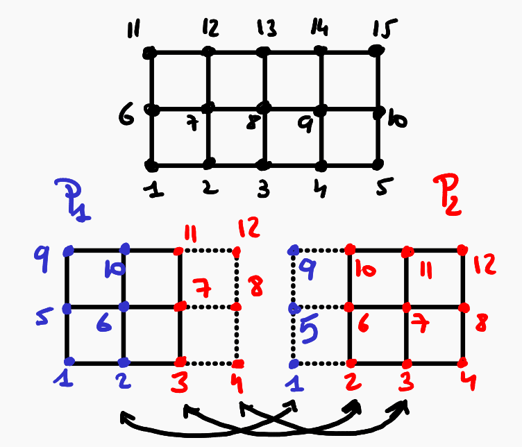
The DoF layout can be seen in the following figure

and can be accessed as follows:
dof_gids = V.gids
local_dofs_to_global_dof = map(local_to_global,partition(dof_gids))
local_dofs_to_owner      = map(local_to_owner,partition(dof_gids))
owned_dofs_to_local_dof  = map(own_to_local,partition(dof_gids))
ghost_dofs_to_local_dof = map(ghost_to_local,partition(dof_gids))We can now define the weak form and integrate as usual:
degree = 2*order
Ω = Triangulation(model)
dΩ = Measure(Ω,degree)

f(x)   = cos(x[1])
a(u,v) = ∫( ∇(v)⋅∇(u) )*dΩ
l(v)   = ∫( v*f )*dΩ

op = AffineFEOperator(a,l,V,U)
uh = solve(op)
Note that by default solve will use the Julia LU direct solver. In parallel, we provide a toy implementation that gathers the whole matrix into a single processor and solves the linear system there. This is not scalable, and should only be used for debugging/testing purposes.
The design of scalable solvers is a very complex issue. Direct factorization solvers such as MUMPS or PARDISO can scale to a few hundred processors, but iterative preconditioned solvers are the only viable option for larger problems.
As we will see in the next tutorial, Gridap provides interfaces to some of the most popular distributed linear algebra libraries, such as PETSc, through satellite packages. We are also in the process of providing Julia-native iterative solvers.
Let's take a moment to have a look at the distributed linear system: As usual, one can access the system matrix and rhs as
A  = get_matrix(op)
b  = get_vector(op)
We observe and are now of type PSparseMatrix and PVector, respectively. These represent distributed equivalents of the serial SparseMatrix and Vector types. Each object holds their local part of the array (both owned and ghost indices) and information on the Owned/Ghost layout for their rows (and columns).
The local sub-matrices and sub-vectors can be accessed as follows:
local_mats = partition(A)
owned_mats = own_values(A)

local_vectors = partition(b)
owned_vectors = own_values(b)
Here, local_mats and local_vectors contain the sub-matrices and sub-vectors for all the local DoFs (owned and ghost, with overlapping between processors), while owned_mats and owned_vectors contain the sub-matrices and sub-vectors for the owned DoFs only (no overlapping).
The row/column layout of the PSparseMatrix can be accessed as follows:
rows = axes(A,1)
cols = axes(A,2)
If we compare them to the DoF layout from the original space , we can see a couple major differences:
owned_dofs_to_local_dof  = map(own_to_local,partition(dof_gids))
ghost_dofs_to_local_dof  = map(ghost_to_local,partition(dof_gids))

owned_rows_to_local_row  = map(own_to_local,partition(rows))
ghost_rows_to_local_row  = map(ghost_to_local,partition(rows))
First, the owned DoFs are not necessarily the first ones in the global ordering. However, owned rows are always the first ones in the global ordering. This reordering is done to comply with the standards set by other distributed linear algebra libraries, such as PETSc.
Second, the number of ghosts in the dof layout is higher than the number of ghosts in the row layout. This is because the row layout only contains the ghosts indices that are needed to compute the local matrix-vector product.
What we take away from this is that we cannot use a PVector of DoFs to solve the linear system and viceversa (which is what we generally do in serial). Moreover, the ghost layout can also be different for the rows and columns. If we ever do this, we will get an error message:
x = get_free_dof_values(uh) # DoF layout
A * x # Error!
A * b # Error!
To allocate PVectors with a specific ghost layout, we can use the function pfill:
x_r = pfill(0.0,partition(axes(A,1))) # Row layout
x_c = pfill(0.0,partition(axes(A,2))) # Col layout
x_r .= A * x_c # OK
Despite this, we can use column and row PVectors to create FEFunctions. The index mapping will be taken care of by GridapDistributed, like so:
vh = FEFunction(V,x_c)